Context
Reproducible research is research for which the numbers reported in the paper can obtained by others using the original data and analysis scripts. (Note that this differs from replicability - the extent to which findings are consistent across samples.) Recent research has revealed a problem with the reproducibility of analyses in many fields. For example, in psychology Nuijten et al. (2015) found that in 50% of articles there was at least once instance of a reported test statistic (e.g., t(24)=22.71) being inconsistent with the reported p-value. This inconsistency rate suggests there is a major problem with reproducibility in the psychological literature.
My objective in creating the apaTables package was to automate the process through which tables are created from analyses when using R. Using apaTables ensures that the tables in your manuscript are reproducible.
Although a number of table generation packages exist for R they are typically not useful for psychology researchers because of the need to report results in the style required by the American Psychological Association; that is, APA Style. Consequently, apaTables creates Microsoft Word documents (.doc files) that contain tables that conform to APA Style.
In many cases it would be necessary to execute additional R commands to obtain all of the statistics needed for an APA Style table. For example, if conducting a regression using the lm command the unstandardized regression (i.e., b) weights are reported. Additional commands are needed to obtain standardized (i.e., beta) weights. apaTables automatically executes these additional commands to create a table with the required information in Microsoft Word .doc format1.
Additionally, the American Statistical Association recently released a position paper on the use of p-values in research. A component of that statement indicated that “Scientific conclusions and business or policy decisions should not be based only on whether a p-value passes a specific threshold.” The Executive Director of the ASA suggested that confidence intervals should be used to interpret data. This statement is consistent with the 1999 position paper from the APA Task Force on Statistical Inference. Consequently, the current version of apaTables indicates significance using stars but more importantly reports confidence intervals for the reported effect sizes.
Bugs and feature requests can be reported at: https://github.com/dstanley4/apaTables/issues
Correlation table
Correlation tables can be constructed using the apa.cor.table() function. The constructed table includes descriptive statistics (i.e., mean and standard deviation) for each variable and a confidence interval for each correlation.
The apa.cor.table() function creates a correlation table with confidence intervals based on a data frame. The example below creates an APA Style correlation table, see Table 1, using the attitude dataset built into R.
library(apaTables)
table1 <- apa.cor.table(attitude,
                        table.number=1)

print(table1)


apa.save(filename = "table1.doc",
         table1)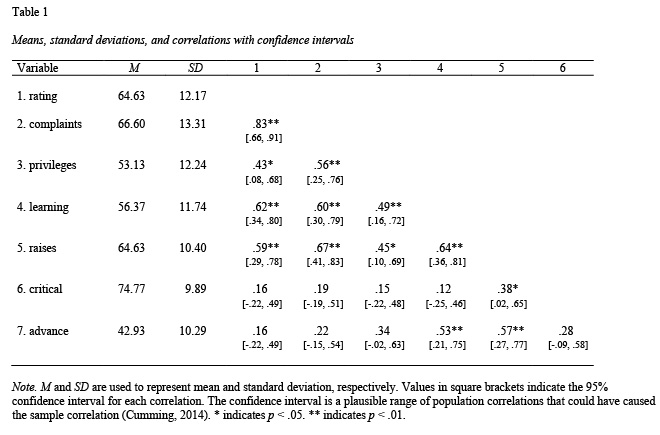
Use the apa.knit.table.for.pdf() function to create a latex table for papaja or Quarto documents:
apa.knit.table.for.pdf(table1)Regression table overview
Regression tables can be constructed using the apa.reg.table() function. The constructed table includes the unstandardized regression coefficient (b with CI), standardized regression coefficient (beta with CI), semi-partial correlation squared ( with CI), the correlation (), and the overall fit of the model (indexed by with CI). The album sales dataset from Field et al. (2012) is used to illustrate the apa.reg.table() function.
Basic regression table
The apa.reg.table() function creates a regression table with confidence intervals based on lm() output; see Table 2.
library(apaTables)

basic.reg <- lm(sales ~ adverts + airplay,
                data = album)

table2 <- apa.reg.table(basic.reg,
                        table.number = 2)

apa.save(filename = "table2.doc",
         table2)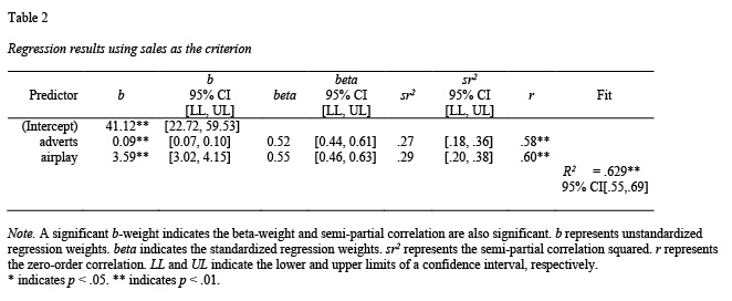
Use the apa.knit.table.for.pdf() function to create a latex table for papaja or Quarto documents:
apa.knit.table.for.pdf(table2)Blocks regression table
In many cases, it is more useful for psychology researchers to compare the results of two regression models with common variables. This approach is known to many psychology researchers as block-based regression (likely due to the labeling used in popular software packages). Using regression to “control” for certain variables (e.g., demographic or socio-economic variables) is a common use case. In this scenario, the researcher conducts a regression with the “control” variables that is referred to as block 1. Following this, the researcher conducts a second regression with the “control” variables and the substantive variables that is referred to as block 2. If block 2 accounts for significant variance in the criterion above and beyond block 1 then substantive variables are deemed to be meaningful predictors.
A second common use of block-based regression in psychology is testing for continuous-variable interactions. Consider a scenario in which a researcher is testing for an interaction between two continuous variables and two regressions are conducted. The first regression includes the two predictors of interest (block 1). The second regression includes the two predictors of interest as well as their product term (block 2). If block 2 accounts for significant variance in the criterion above and beyond block 1 an interaction is deemed to be present. Admittedly interactions could be tested in a single regression; however, using a block-based regression for this analysis is common in psychology. The example below examines whether advertisements and amount of airplay for a song interact to predict album sales. The resulting table is presented in Table 3. Although this example only uses two blocks, note that any number of blocks can be used with the apa.reg.table() function. As well, if the predictors in any of the blocks are a product-term, the zero-order correlation will be omitted from the output to prevent interpretation errors common in psychology.
The apa.reg.table() function allows for multiple (i.e., more 2 or more) blocks as per below; see Table 3.
library(apaTables)

block1 <- lm(sales ~ adverts + airplay, data = album)
block2 <- lm(sales ~ adverts + airplay + I(adverts*airplay), data = album)

table3 <- apa.reg.table(block1, block2,
                        table.number = 3)

apa.save(filename = "table3.doc",
         table3)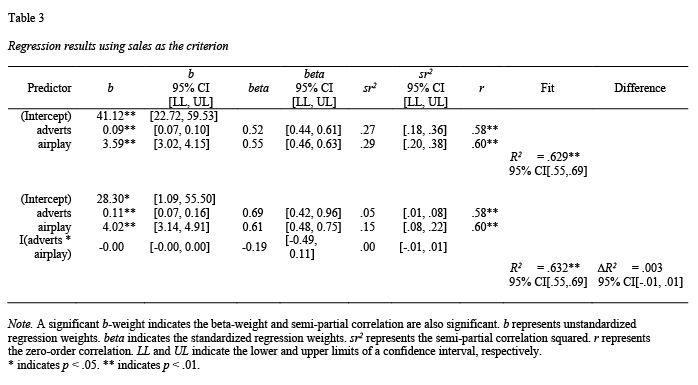
Use the apa.knit.table.for.pdf() function to create a latex table for papaja or Quarto documents:
apa.knit.table.for.pdf(table3)1-way ANOVA and d-value tables
There are three functions in apaTables that are helpful for 1-way ANOVA analyses within predictor variables that are independent (apa.aov.table(), apa.1way.table(), and apa.d.table()). All three are illustrated below. First, however, the ANOVA must be conducted - we do so using the viagra dataset from Field et al. (2012). When conducting an ANOVA in R using the lm() command you must ensure your independent variables are R factors and that contrasts are set correctly. Note: repeated measures designs are supported via the apa.ezANOVA.table() command.
The apa.aov.table() function creates a 1-way ANOVA table based on lm_output; see Table 4.
library(apaTables)

table4 <- apa.aov.table(lm_output,
                        table.number = 4)

apa.save(filename = "table4.doc",
         table4)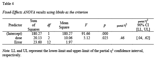
Use the apa.knit.table.for.pdf() function to create a latex table for papaja or Quarto documents:
apa.knit.table.for.pdf(table4)The apa.1way.table() function creates a table with the mean and sd for each cell; see Table 5.
table5 <- apa.1way.table(iv = dose,
                         dv = libido,
                         data = viagra,
                         table.number = 5)

apa.save(filename = "table5.doc",
         table5)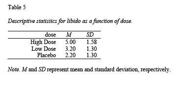
Use the apa.knit.table.for.pdf() function to create a latex table for papaja or Quarto documents:
apa.knit.table.for.pdf(table5)The apa.d.table() function show a d-value (with confidence interval) for each paired comparison; see Table 6.
table6 <- apa.d.table(iv = dose,
                      dv = libido,
                      data = viagra,
                      table.number = 6)

apa.save(filename = "table6.doc",
         table6)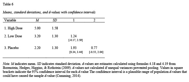
Use the apa.knit.table.for.pdf() function to create a latex table for papaja or Quarto documents:
apa.knit.table.for.pdf(table6)N-way ANOVA tables: 2-way Example
The 2-way example with independent variable predictors is based on the goggles dataset from Field et al. (2012). As before, when conducting an ANOVA in R using the lm() command you must ensure your independent variables are R factors and that contrasts are set correctly. Note: repeated measures designs are supported via the apa.ezANOVA.table() command.
options(contrasts = c("contr.sum", "contr.poly"))

lm_output <- lm(attractiveness ~ gender*alcohol,
                data = goggles)
The apa.aov.table() function creates a 2-way ANOVA table based on lm_output; see Table 7.
library(apaTables)

table7 <- apa.aov.table(lm_output,
                        table.number = 7)

apa.save(filename = "table7.doc",
         table7)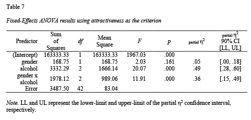
Use the apa.knit.table.for.pdf() function to create a latex table for papaja or Quarto documents:
apa.knit.table.for.pdf(table7)The apa.2way.table() function creates a table with the mean and sd for each cell; see Table 8. Marginal means can also be requested with the show.marginal.means = TRUE. For higher-order designs (i.e., 3-way or higher) use the filter() command in the tidyverse package to select the subset of rows and then use apa.2way.table() to display cell statistics.
table8 <- apa.2way.table(iv1 = gender,
                         iv2 = alcohol,
                         dv = attractiveness,
                         data = goggles,
                         show.marginal.means = TRUE,
                         table.number = 8)

apa.save(filename = "table8.doc",
         table8)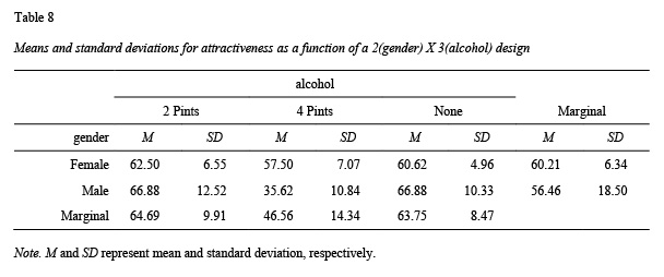
Use the apa.knit.table.for.pdf() function to create a latex table for papaja or Quarto documents:
apa.knit.table.for.pdf(table8)You can use the tidyverse package to conducted paired comparisons within each gender again using apa.d.table(); see Tables 9 and 10.
library(apaTables)

library(dplyr)

goggles.men   <- filter(goggles,gender=="Male")
goggles.women <- filter(goggles,gender=="Female")

table9 <- apa.d.table(iv = alcohol,
                      dv = attractiveness,
                      data = goggles.men,
                      table.number = 9)

table10 <- apa.d.table(iv = alcohol,
                       dv = attractiveness,
                       data = goggles.women,
                       table.number = 10)

apa.save(filename = "tables9and10.doc",
         table9, table10)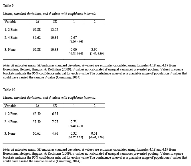
Use the apa.knit.table.for.pdf() function to create a latex table for papaja or Quarto documents:
apa.knit.table.for.pdf(table9)
apa.knit.table.for.pdf(table10)
ezANOVA and apaTables: Repeated measures ANOVA
apaTables also supports repeated measures ANOVA tables and repeated measures by between measures (mixed) ANOVA tables via ezANOVA output from the ez package.
Repeated Measures: 2-way design
Prior to begining we ‘open’ the apaTables, tidyverse, and ez packages using the library command as per below.
In this example, we used the drink_attitude dataset from Field et al. (2012). As before, this dataset is built into apaTables so it does not need to be loaded using read_csv() or read_sav(). The dataset (drink_attitude_wide) can be inspected with the glimpse() command below (this provides information similar to SPSS variable view). We use the “wide” descriptor in the name of the dataset to remind us that the data is in in the “wide” format where one row contains all the data for one person. There are 20 participants so there are 20 rows.
glimpse(drink_attitude_wide)The dataset represents an ANOVA with two repeated measures factors. It is a 3 drinks (wine, beer, water) X 3 imagery (positive, negative, neutral) design. The dataset uses 10 columns to represent this design. The first column contains a code for each participant (P1, P2, etc.) Note that the participant column is a factor as indicated by the < fctr > descriptor. The participant column must be a factor which can, as noted previously, be created by the as_factor() command.
Each of the remaining 9 columns contain atittude ratings for a single drink/imagery combination cell. The naming convention for column names is critical to the workflow we describe below. Each column name represents the level of the drink variable separated using an underscore ( _ ) from a level of the imagery variable. For example the first column is called beer_positive representing the cell with a combination of the the beer level of drink and the positive level of imagery. Each value in this column represents attitude for a participant in this cell.
In order to conduct a repeated measures ANOVA we need to convert the dataset from the wide format (where each row represents a person) to the long format (where each row represents a single observation from a person). We do this with a series of commands below.
drink_attitude_long <- tidyr::pivot_longer(drink_attitude_wide,
                              cols = beer_positive:water_neutral,
                              names_to = c("drink", "imagery"),
                              names_sep = "_",
                              values_to = "attitude")


drink_attitude_long$drink <- as_factor(drink_attitude_long$drink)
drink_attitude_long$imagery <- as_factor(drink_attitude_long$imagery)
We can inspect the final long version of the dataset with glimpse again:
glimpse(drink_attitude_long)This output reveals the new data structure. There are now only four columns where each row represents a single observation for a participant. As before, the first column is factor column representing participant. But each participant is represented nines times in this column now - because each participant has nine observations (i.e., one in each of the nine cells). Most importantly, we now have a single column indicating level of drink, a single column indicating level of imagery, and a column indicating the attitude rating.
You can see the first few rows in the more familiar format below:
head(drink_attitude_long)Prior to conducting the analysis we set the contrasts as per Field et al. (2012).
alcohol_vs_water <- c(1, 1, -2)
beer_vs_wine <- c(-1, 1, 0)
negative_vs_other <- c(1, -2, 1)
positive_vs_neutral <- c(-1, 0, 1)
contrasts(drink_attitude_long$drink) <- cbind(alcohol_vs_water, beer_vs_wine)
contrasts(drink_attitude_long$imagery) <- cbind(negative_vs_other, positive_vs_neutral)
Then we use the ezANOVA command from the ez package to conduct the repeated measures ANOVA. Be sure to include all of the commands below including the options command which ensures that the output has sufficent number of digits (i.e., numbers after the decimal) for apaTables.
options(digits = 10)

drink_attitude_results <- ezANOVA(data = drink_attitude_long,
                                  dv = .(attitude),
                                  wid = .(participant),
                                  within = .(drink, imagery),
                                  type = 3,
                                  detailed = TRUE)
Now we make the table based on the output:
table11 <- apa.ezANOVA.table(drink_attitude_results,
                             table.number = 11)

apa.save(filename = "table11.doc",
         table11)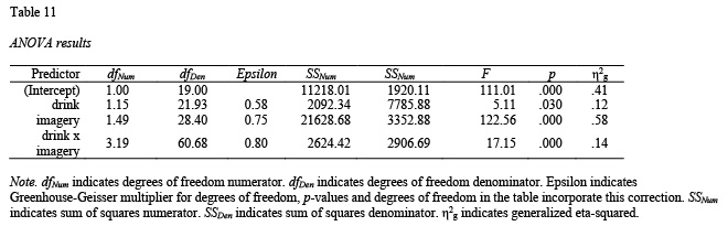
Use the apa.knit.table.for.pdf() function to create a latex table for papaja or Quarto documents:
apa.knit.table.for.pdf(table11)Repeated Measures and Independent Groups: 3-way design
Prior to begining we ‘open’ the apaTables, tidyverse, and ez packages using the library command as per below.
In this example, we used the drink_attitude dataset from Field et al. (2012). As before, this dataset is built into apaTables. The dataset (dating_wide) can be inspected with the glimpse() command below (this provides information similar to SPSS variable view). We use the “wide” descriptor in the name of the dataset to remind us that the data is in in the “wide” format where one row contains all the data for one person. There are 20 participants so there are 20 rows.
glimpse(dating_wide)The dataset represents an ANOVA with one independent groups factor and two repeated measures factors. It is a 2 gender (male, female) by 3 looks (attrative, average, ugly) X 3 personality (high, some, none) design. The dataset uses 11 columns to represent this design. The first column contains a code for each participant (P1, P2, etc.) Note that the participant column is a factor as indicated by the “< fctr >” descriptor. The second column is used to indicate the gender of each participant. Both the participant and gender columns are factors.
Each of the remaining 9 columns contain atittude ratings for a single looks/personality combination cell. The naming convention for column names is critical to the workflow we describe below. Each column name represents the level of the looks variable separated using an underscore ( _ ) from a level of the personality variable. For example the first column is called attractive_high representing the cell with a combination of the the attractive level of looks and the high level of personality. Each value in this column represents date rating for a participant in this cell.
In order to conduct a mixed between/within ANOVA we need to convert the dataset from the wide format (where each row represents a person) to the long format (where each row represents a single observation from a person) – taking into account the independent groups factors (gender). We do this with a series of commands below.
dating_long <- tidyr::pivot_longer(dating_wide,
                                   cols = attractive_high:ugly_none,
                                   names_to = c("looks", "personality"),
                                   names_sep = "_",
                                   values_to = "date_rating")


dating_long$looks <- as_factor(dating_long$looks)
dating_long$personality <- as_factor(dating_long$personality)
We can inspect the final long version of the dataset with glimpse again:
glimpse(dating_long)This output reveals the new data structure. There are now only five columns where each row represents a single observation for a participant. As before, the first column is factor column representing participant. But each participant is represented nines times in this column now - because each participant has nine observations (i.e., one in each of the nine cells). The second column contains the gender factor. The third column indicates the level of looks, and the fourth column indicates the level of personality. The fith column indicates the date_rating.
You can see the first few rows in the more familiar format below:
head(dating_long)Prior to conducting the analysis we set the contrasts as per Field et al. (2012).
some_vs_none <- c(1, 1, -2)
hi_vs_av <- c(1, -1, 0)
attractive_vs_ugly <- c(1, 1, -2)
attractive_vs_average <- c(1, -1, 0)
contrasts(dating_long$personality) <- cbind(some_vs_none, hi_vs_av)
contrasts(dating_long$looks) <- cbind(attractive_vs_ugly, attractive_vs_average)
Then we use the ezANOVA command from the ez package to conduct the repeated measures ANOVA. Be sure to include all of the commands below including the options command which ensures that the output has sufficent number of digits (i.e., numbers after the decimal) for apaTables.
options(digits = 10)
dating_results <-ezANOVA(data = dating_long,
                         dv = .(date_rating),
                         wid = .(participant),
                         between = .(gender),
                         within = .(looks, personality),
                         type = 3,
                         detailed = TRUE)
Now we make the table based on the output:
table12 <- apa.ezANOVA.table(dating_results,
                                  filename = "Table12_APA.doc",
                                  table.number = 12)

apa.save(filename = "table12.doc",
         table12)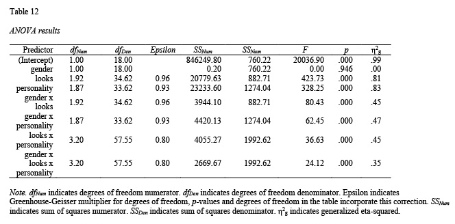
Use the apa.knit.table.for.pdf() function to create a latex table for papaja or Quarto documents:
apa.knit.table.for.pdf(table12)References
Field, A., Miles, J., Field, Z. Discovering statistics using R. Sage: Chicago.
Nuijten, M. B., Hartgerink, C. H. J., van Assen, M. A. L. M., Epskamp, S., & Wicherts, J. M. (2015). The prevalence of statistical reporting errors in psychology (1985-2013). Behavior Research Methods. http://doi.org/10.3758/s13428-015-0664-2