print( var(true) )[1] 100print( var(observed) )[1] 125rxx = var(true) / var(observed)
print( rxx )[1] 0.8Part 1: \(r_{xx} = \frac{\sigma_{\text{true}}^2}{\sigma_{\text{observed}}^2}\)
print( var(true) )[1] 100print( var(observed) )[1] 125rxx = var(true) / var(observed)
print( rxx )[1] 0.8Part 2: \(\sqrt{r_{xx}} = \frac{\sigma_{\text{true}}}{\sigma_{\text{observed}}}\)
print( sqrt(rxx) )[1] 0.8944272print( sd(true) / sd(observed) )[1] 0.8944272\(\sigma_{\text{observed}}^2r_{xx} = \sigma_{\text{true}}^2\)
print( rxx * var(observed) )[1] 100print( var(true) )[1] 100Part 1: \(r_{xx} = r_{\text{(observed, true)}}^2\)
print( rxx )[1] 0.8print( cor(observed, true)^2 )[1] 0.8Part 2: \(\sqrt{r_{xx}} = r_{\text{(observed, true)}}\)
print( sqrt(rxx) )[1] 0.8944272print( cor(observed, true) )[1] 0.8944272\(r_{xx}= 1 - \frac{\sigma_{\text{error}}^2}{\sigma_{\text{observed}}^2}\)
print( rxx )[1] 0.8print( 1 - var(error)/var(observed) )[1] 0.8\(\overline{\text{true}} = \overline{\text{observed}}\)
print( mean(true) )[1] 100print( mean(observed) )[1] 100We make a regression predicting \(y\) using \(x\) with the code below. Notice the regression line has a slope of .80 and an intercept of 20.
# Will use the generic labels of y and x in the regression demonstration
# We create variables with these labels
y <- true
x <- observed

# Create the regression model relating x to y using the lm() command. lm() is linear model.
my_model <- lm(y ~ x)
print(my_model)
Call:
lm(formula = y ~ x)

Coefficients:
(Intercept)            x
20.0 0.8 We graph the relation between \(x\)-values and \(y\)-values with the code below. We include the regression line described in the output above using the geom_smooth() command. Warning: This make take a few minutes to plot.
# Create a data frame (spreadsheet style) version of the data
my_df <- data.frame(y, x)

# Plot the data and use geom_smooth()
# to show regression line
ggplot(data = my_df,
       mapping = aes(x = x,
                     y = y)) +
  geom_point(color = "grey") +
  geom_smooth(method = lm,
              formula = y ~ x,
              color = "blue") +
  theme_classic(18)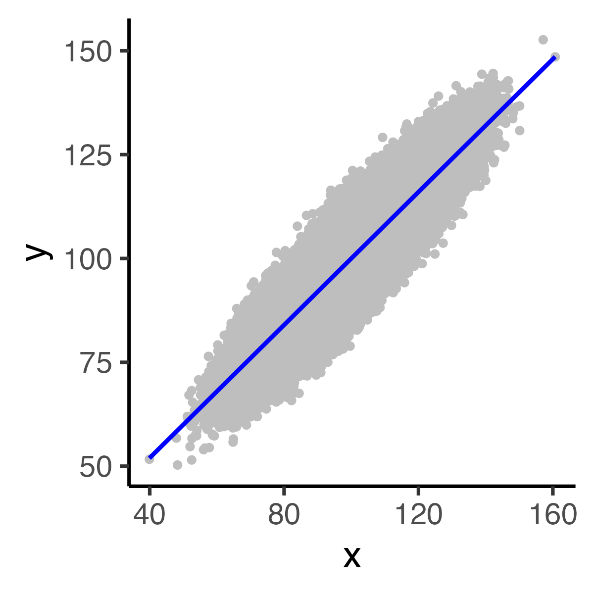
Using \(x=120\) we create a predicted value for \(y\) (i.e., a \(\hat{y}-value\)) for the graph above. This predicted value is the spot on the regression line above \(x=120\). We do so with knowledge of the full regression equation, including the intercept.
b = 0.80 # the slope
intercept = 20
yhat = b*(120) + intercept
print(yhat)
[1] 116A predicted value can be created without a regression equation - as explained in the paper. As before, using \(x=120\) we create a predicted value for \(y\) (i.e., a \(\hat{y}-value\)) for the graph above. We do so WITHOUT knowledge of the full regression equation - we do not know the intercept but we do know the mean of \(x\) and the mean of \(y\). The regression line will always run through the point (\(\bar{x}, \bar{y}\)) - so this is used as a frame of reference. Because we do not know true scores in an applied context, we use this approach to generated predicted values for measurement intervals.
b = 0.80 # the slope
yhat = mean(y) + b*(120 - mean(x))
print(yhat)
[1] 116The predicted value of \(y\) (i.e., \(\hat{y}-value\)) is an estimate of the mean value of \(y\) for those test takers with the specified value of \(x\). In this example \(x = 120\). For participants with score of 120 on the \(x\)-axis we calculate the mean value of their \(y\) scores. We see the resulting mean is the same as the \(\hat{y}-value\) above.
people_with_x_equal_120 <- round(x) == 120

# mean y-value for these people
print( mean( y[people_with_x_equal_120] ) )
[1] 115.9464In the previous step, we estimated a mean \(y\)-value as \(\hat{y}=116\) for people with an observed score of 120. In this simulation we correspondingly found a mean \(y\)-value of 116 (rounded).
Notice in the output below that residual standard error is 4.47. This value is the standard deviation of the residuals around the regression line.
summary(my_model)
Call:
lm(formula = y ~ x)

Residuals:
     Min       1Q   Median       3Q      Max
-20.8089  -3.0177  -0.0016   3.0176  21.6884

Coefficients:
            Estimate Std. Error t value Pr(>|t|)
(Intercept) 20.00000    0.04025   496.9   <2e-16 ***
x            0.80000    0.00040  2000.0   <2e-16 ***
---
Signif. codes:  0 '***' 0.001 '**' 0.01 '*' 0.05 '.' 0.1 ' ' 1

Residual standard error: 4.472 on 999998 degrees of freedom
Multiple R-squared:    0.8, Adjusted R-squared:    0.8
F-statistic: 4e+06 on 1 and 999998 DF,  p-value: < 2.2e-16
We can obtain the same 4.47 value using the equation below. This equation is central to the derivation of the error equations for Standard Error of Estimation and Standard Error of Measurement.
yhat_residual_sd_everyone = sd(y) * sqrt(1 - cor(x,y)^2)

print(yhat_residual_sd_everyone)
[1] 4.472136