rxx = var(true)/var(observed)
print(rxx)
[1] 0.8In this section, with the Standard Error of Estimation (SEE), we create a 95% SEE regression interval that will capture 95% of the true scores for test takers with the same observed score. In this demonstration we create a 95% SEE interval based on an observed score of 90.
Again note that in an applied context, we do not know true score so a regression model like the one below cannot be created. This regression model between true score and observed scores is a presented as a way to understand the conceptual basis for the Standard Error of Estimation interval.
Previously, we created true scores and errors as data for this demonstration. Recall that the reliability of these observed scores is \(r_{xx}=.80\).
rxx = var(true)/var(observed)
print(rxx)[1] 0.8Now we create the Standard Error of Estimation regression model. In this model, observed scores predict true scores. Notice the slope corresponds to the reliability in the Standard Error of Estimation regression model. This correspondence between slope and reliability does not occur with the Standard Error of Measurement regression model.
see_model <- lm(true ~ observed)
print(see_model)
Call:
lm(formula = true ~ observed)

Coefficients:
(Intercept)     observed
       20.0          0.8
This output above indicates the regression equation:
\[ \hat{y}_{true} = .80(x_{observed}) + 20 \]
We graph the relation between observed scores and true scores with the code below. Warning: This make take a few minutes to plot.
# view model and predicted values
library(ggplot2)
example_df <- data.frame(true, observed)

ggplot(data = my_df,
       mapping = aes(x = observed,
                     y = true)) +
  geom_point(color = "grey") +
  geom_smooth(method = lm,
              formula = y ~ x,
              color = "blue") +
  ggtitle("SEE Regression Model") +
  scale_x_continuous(breaks = seq(50, 150, by = 20)) +
  theme_classic()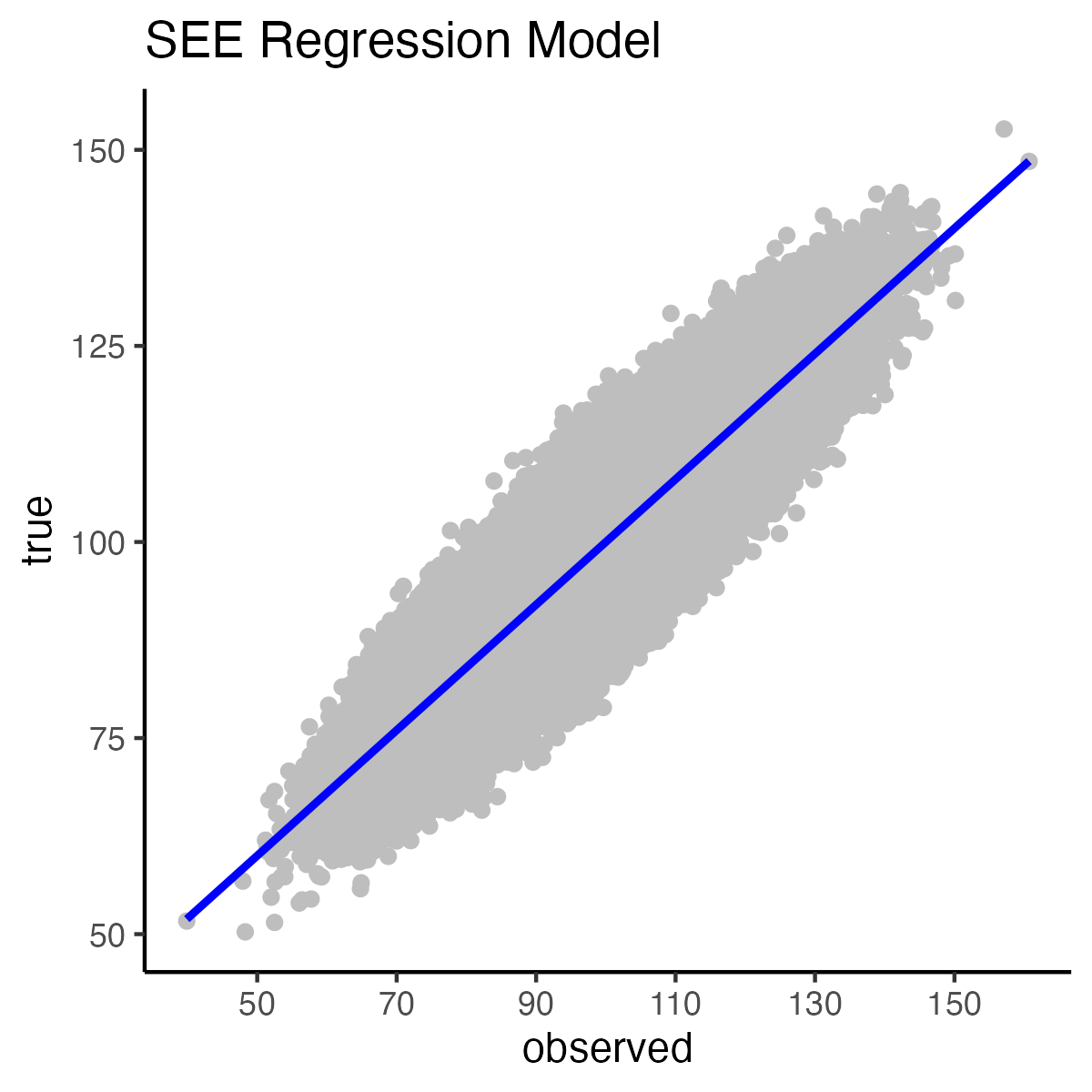
The output above indicated the regression equation:
\[ \hat{y}_{true} = .80(x_{observed}) + 20 \]
This equation equation is used to generate the values on the regression line in graph above. Example calculation for a spot on the regression line corresponding to an observed score of 90:
\[ \begin{aligned} \hat{y}_{true} &= .80(x_{observed}) + 20\\ &= .80(90) + 20\\ &= 92 \end{aligned} \]
This predicted value is an estimate of the mean true score for those test takers with an observed score of 90.
Keep in mind, however, that in a applied measurement context, don’t know true scores. Consequently, we cannot generate a regression between true scores and observed scores. This means we don’t know the intercept in the regression equation. As a result, in any applied context we will not have have the full regression equation so this calculation is not possible.
In an applied measurement context, we will know the reliability and the mean of the observed scores. This allows us to use an alternative approach to create \(\hat{y}_{true}\)-values.
We create a predicted true score (i.e., \(\hat{y}_{true}\)) based on an observed score, the mean observed score, and the reliability (i.e., slope):
\[ \hat{y}_{true} = \overline{observed} + r_{xx} (observed - \overline{observed}) \]
We obtain a predicted true score (i.e., \(\hat{y}-value\)) of approximately 92 using the equation below based on an observed score of 90. Again, this predicted value is an estimate of the mean true score for those test takers with an observed score of 90.
yhat = mean(observed) + rxx*(90 - mean(observed))
print(yhat)
[1] 92When we create a Standard Error of Estimation interval for test takers, based on an observed score of 90, it is centered on \(\hat{y}=92\).
This spot on the regression line is illustrated in the graph below by the red dot:
# view model and predicted values
library(ggplot2)
example_df <- data.frame(true, observed)

ggplot(data = my_df,
       mapping = aes(x = observed,
                     y = true)) +
  geom_point(color = "grey") +
  geom_smooth(method = lm,
              formula = y ~ x,
              color = "blue") +
  ggtitle("SEE Regression Model") +
  scale_x_continuous(breaks = seq(50, 150, by = 20)) +
  theme_classic() +
  annotate(geom = "point",
           x = 90, y = 92,
           color = "red", size = 4)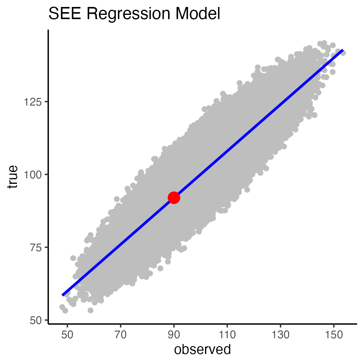
The length of the interval depends on the standard deviation of the residuals around the corresponding spot on the regression line (i.e., the red dot in the graph above). Due to the homoscedasticity assumption the standard deviation of the residuals at that point is equal to the overall standard deviation of the residuals. We obtain the overall standard deviation of the residuals in R output by looking at “Residual Standard Error”. Notice that this value is 4.47 in the output below.
summary(see_model)
Call:
lm(formula = true ~ observed)

Residuals:
     Min       1Q   Median       3Q      Max
-20.8089  -3.0177  -0.0016   3.0176  21.6884

Coefficients:
            Estimate Std. Error t value Pr(>|t|)
(Intercept) 20.00000    0.04025   496.9   <2e-16 ***
observed     0.80000    0.00040  2000.0   <2e-16 ***
---
Signif. codes:  0 '***' 0.001 '**' 0.01 '*' 0.05 '.' 0.1 ' ' 1

Residual standard error: 4.472 on 999998 degrees of freedom
Multiple R-squared:    0.8, Adjusted R-squared:    0.8
F-statistic: 4e+06 on 1 and 999998 DF,  p-value: < 2.2e-16
Notice that we can get an estimate of this value from the SEE-error formula. We use the value below in our Standard Error of Estimation interval calculation.
sd_residual_see = sd(observed)*sqrt( (1-rxx)*rxx)
print(sd_residual_see)
[1] 4.472136Recall, we started with the intent to make a Standard Error of Estimation interval based on an observed score of 90. Using this, in the above activities, we estimated \(\hat{y}\) (the center of the interval) and \(s_{residual}\) which determined the length of the interval:
print(yhat)[1] 92print(sd_residual_see)[1] 4.472136We use these values to calculate the lower limit of the interval:
seeLL = yhat - 1.96 * sd_residual_see
print(seeLL)
[1] 83.23461Likewise we calculate the upper limit of the interval:
seeUL = yhat + 1.96 * sd_residual_see
print(seeUL)
[1] 100.7654The result is the 95% SEE [83.23, 100.77] interval. This interval is a range that indicates that for those test takers with an observed score of 90 that 95% of them have true scores between 83.23 and 100.77.
# view model and predicted values
library(ggplot2)
my_df <- data.frame(true, observed)

ggplot(data = my_df,
       mapping = aes(x = observed,
                     y = true)) +
  geom_point(color = "grey") +
  geom_smooth(method = lm,
              formula = y ~ x,
              color = "blue") +
  ggtitle("SEE Regression Model") +
  scale_x_continuous(breaks = seq(50, 150, by = 20)) +
  theme_classic() +
  annotate(geom = "point",
           x = 90, y = 92,
           color = "red", size = 4) +
  annotate(geom = "segment",
           x = 90, xend = 90,
           y = 83.23, yend = 100.77,
           color = "red", linewidth = 1)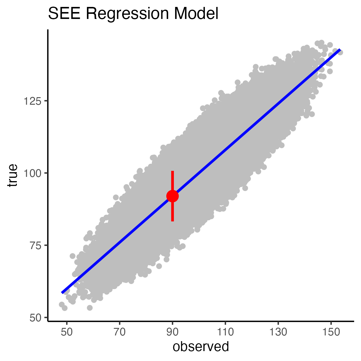
Unfortunately, the above graph makes it appear the 95% SEE interval falls far short of capturing 95% of the true scores corresponding to the \(x-axis\) observed score location of 90. This is occurs because the above plot does not convey the density of the points in the cross section where the interval falls on the graph.
However, if we take a cross section of the data at this point, we can see the interval does capture 95% of the points at this spot on the graph.
people_with_obs_equal_90 <- round(observed) == 90

my_df_hist <- data.frame(true_scores = true[people_with_obs_equal_90])

ggplot(data = my_df_hist,
       mapping = aes(x =true_scores)) +
  geom_histogram() +
  xlab("Trues Scores for People With Observed = 90") +
  ylab("Frequency") +
  scale_x_continuous(breaks = seq(60, 110, by = 2)) +
  ggtitle("SEE Regression Model: Cross Section") +
  theme_classic() +
  annotate(geom = "point",
           x = 92, y = 100,
           color = "red", size = 4) +
  annotate(geom = "segment",
           y = 100, yend = 100,
           x = 83.23, yend = 100.77,
           color = "red", linewidth = 1)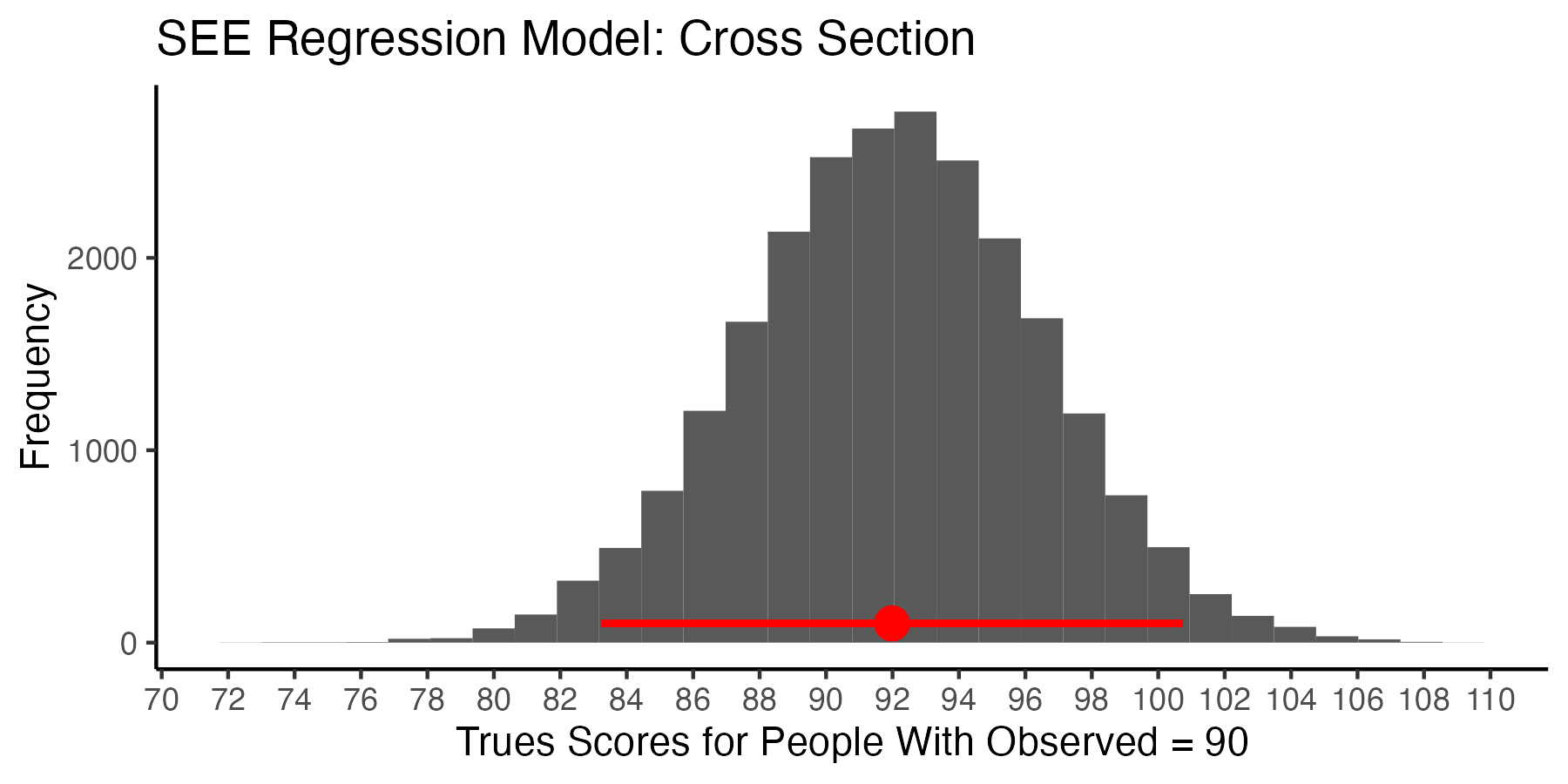
A visual inspection suggest the interval does capture 95% of values. We can confirm our visual inspection of the above graph with a calculation:
people_with_obs_equal_90 <- round(observed) == 90
true_scores_people_with_obs_equal_90 = true[people_with_obs_equal_90]
n_true_scores_for_obs_90 = length(true_scores_people_with_obs_equal_90)

boolean_greater_LL  <- true_scores_people_with_obs_equal_90 >= seeLL
boolean_less_UL     <- true_scores_people_with_obs_equal_90 <= seeUL
boolean_in_interval <- boolean_greater_LL & boolean_less_UL

n_in_interval = sum(boolean_in_interval)
percent_true_in_interval = n_in_interval / n_true_scores_for_obs_90 * 100

print(percent_true_in_interval)
[1] 95.06885Thus, the 95% SEE [83.24, 100.74] captures 95% of the true scores for individuals with an observed score of 90.