Chapter 13 Positive Predictive Value
13.2 Overview
Typically when students learn about p-values and Null Hypothesis Significance testing they tend to pair two ideas. Specifically, they tend to pair a significant \(p\)-value with the idea there is an effect. The purpose of this section is to unpair those two ideas. Specifically, a significant \(p\)-value only indicates that there may be an effect.
At this point you’ve learned to be cautious when it comes to interpreting \(p\)-values. But so far, that’s been more of a qualitative form of caution. In this section we attempt to make it a more quantitative form of caution. Specifically, we introduce you to the concept of positive predictive values (PPV) in the context of interpreting significant p-values. The PPV statistic provides us with an estimate of how likely it is there really is an effect when a p-value is significant. The approach for this chapter was inspired by a blog post. I strongly encourage you to watch this video by the Center for Open Science on the consequences of low statistical power.
13.3 Informal explanation
13.3.1 Probability of an effect
When you conduct an experiment to determine if an effect exists you start off fairly confident that the effect is there - otherwise you would not invest the time and money to run the study. But some research hypotheses will be true and others will not be true. One way to think about this is by imagining 1000 hypothesis as per Figure 13.1. In this figure there are 1000 squares. Each square represents an hypothesis worth testing. Just like the real world some hypotheses are true and some are false. We’ve shaded the squares to indicate which hypotheses are true or false. More specifically, we shaded 40% of the 1000 hypotheses (i.e., 400) green to indicate they are true (i.e., there is an effect). In contrast, we shaded 60% of the 1000 hypotheses (i.e., 600) yellow to indicate they are false (i.e., there is no effect).
Why did we pick the percentage of hypotheses that are true in Figure 13.1 to be 40%? We did so because 40% could well correspond to the number of hypotheses that are true in psychology research overall. It’s difficult to assess the number of hypotheses that are true in psychology given that there is a tendency for only significant effects to be published. However, we can examine pre-registered studies to obtain an estimate of the percentage of hypotheses that are true. With pre-registration scientists register their hypotheses before they collect their data. Consequently looking at the percentage of pre-registered hypotheses that are true may be a reasonable estimate of the percentage of hypotheses that are true in general. Fortunately, a recent study examined a large set of pre-registered studies and determined that just over 40% of research hypotheses are true (Scheel, Schijen, and Lakens 2020). This finding correspondingly implies that approximately 60% of research hypotheses are false. That is, approximately 60% of studies fail to find the desired effect. We used these percentages to shade Figure 13.1. More specifically, we used these numbers to indicate P(effect) = .400 and the P(no effect) = .600.

FIGURE 13.1: One-thousand hypotheses represented as squares. True hypotheses are indicated by the color green. False hypotheses are indicated by the color yellow.
13.3.2 Type I Error
Even when an hypothesis is false there still a chance we will obtain a significant result (i.e., \(p\) < .05). More specifically, we will obtain a significant result 5% of the time when the null hypothesis is true and there is no effect (i.e., \(\alpha = .05\)). In terms of our example, this means that of the 600 false hypotheses, we would obtain a significant result for 30 of them (i.e., .05 * 600 = 30). These 30 false positive significance tests are illustrated in Figure 13.2 below.
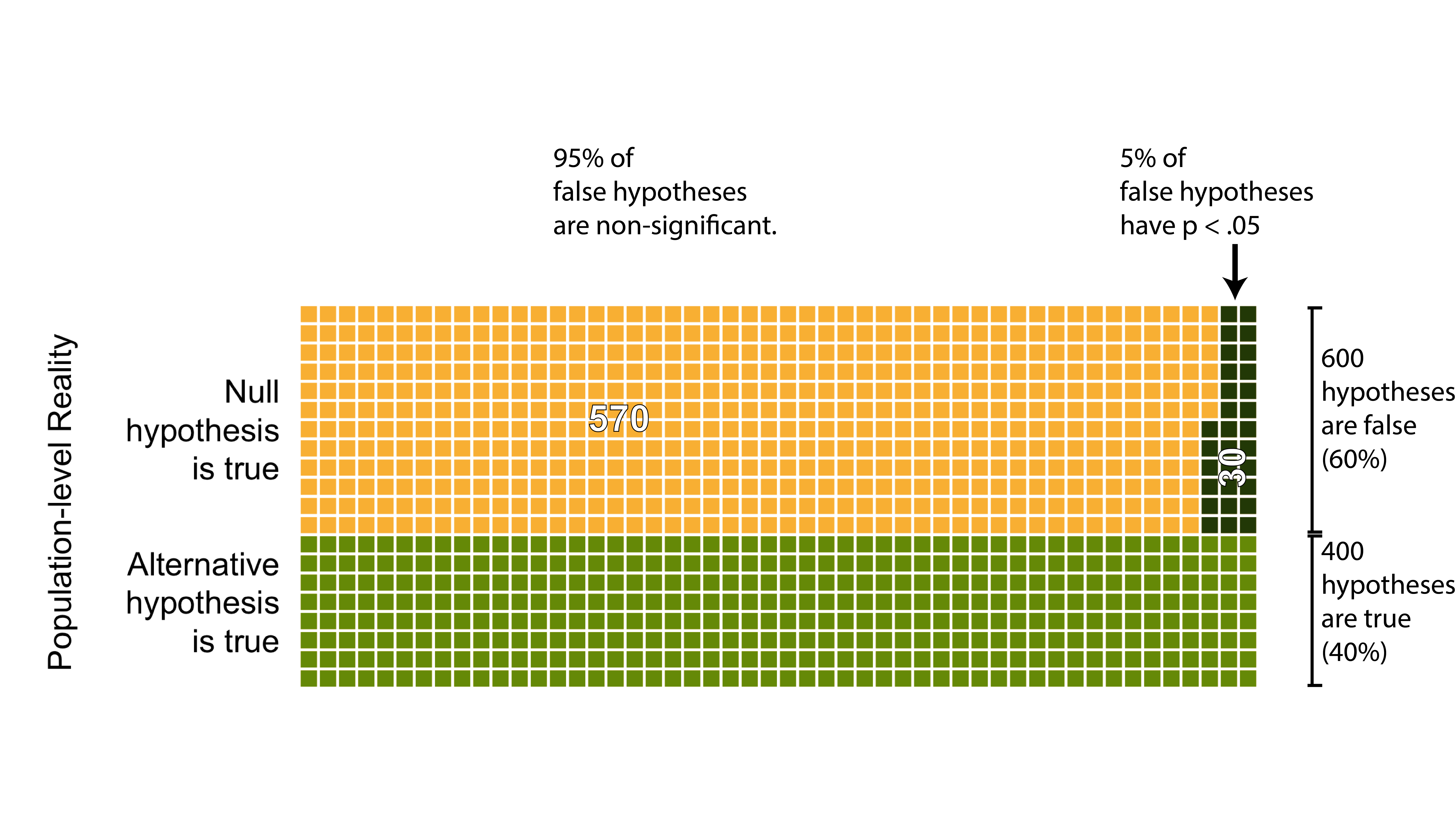
FIGURE 13.2: False positive significance tests. False hypotheses for which the researcher obtained a significant result are indicated by dark green squares.
13.3.3 Power
Unfortunately, even when an hypothesis is true we won’t always obtain a significant p-value. Low sample sizes in psychology are common. As a result most studies in psychology only have a 30% chance of finding an effect if there is one. That is, the typical value for statistical power in psychology is around .30. This typical statistical power level is illustrated in the context of our example in Figure 13.3 below. In this figure, hypotheses that were true but obtained non-significant p-values are indicated by red squares. In contrast, the hypotheses that were true and obtained significant p-values are indicated by green squares; there are 120 green squares.

FIGURE 13.3: True positive signficance tests. True hypotheses for which the researcher obtained a significant result are indicated by green squares. True hypotheses for which the researcher obtained a non-significant result are indicated by red squares.
13.3.4 Calculating PPV
You can see from the blue outline in Figure 13.4, below, that there two ways to obtain a significant p-value. Specifically, you can obtain a significant p-value when the null hypothesis is true (a false positive p-value). As well, you can obtain a significant p-value when the null hypothesis is false (a true positive p-value). As a researcher, when we obtain a significant p-value we don’t know if it’s a true-positive or a false-positive. We calculate PPV to determine how likely it is there is an effect when the p-value is significant.
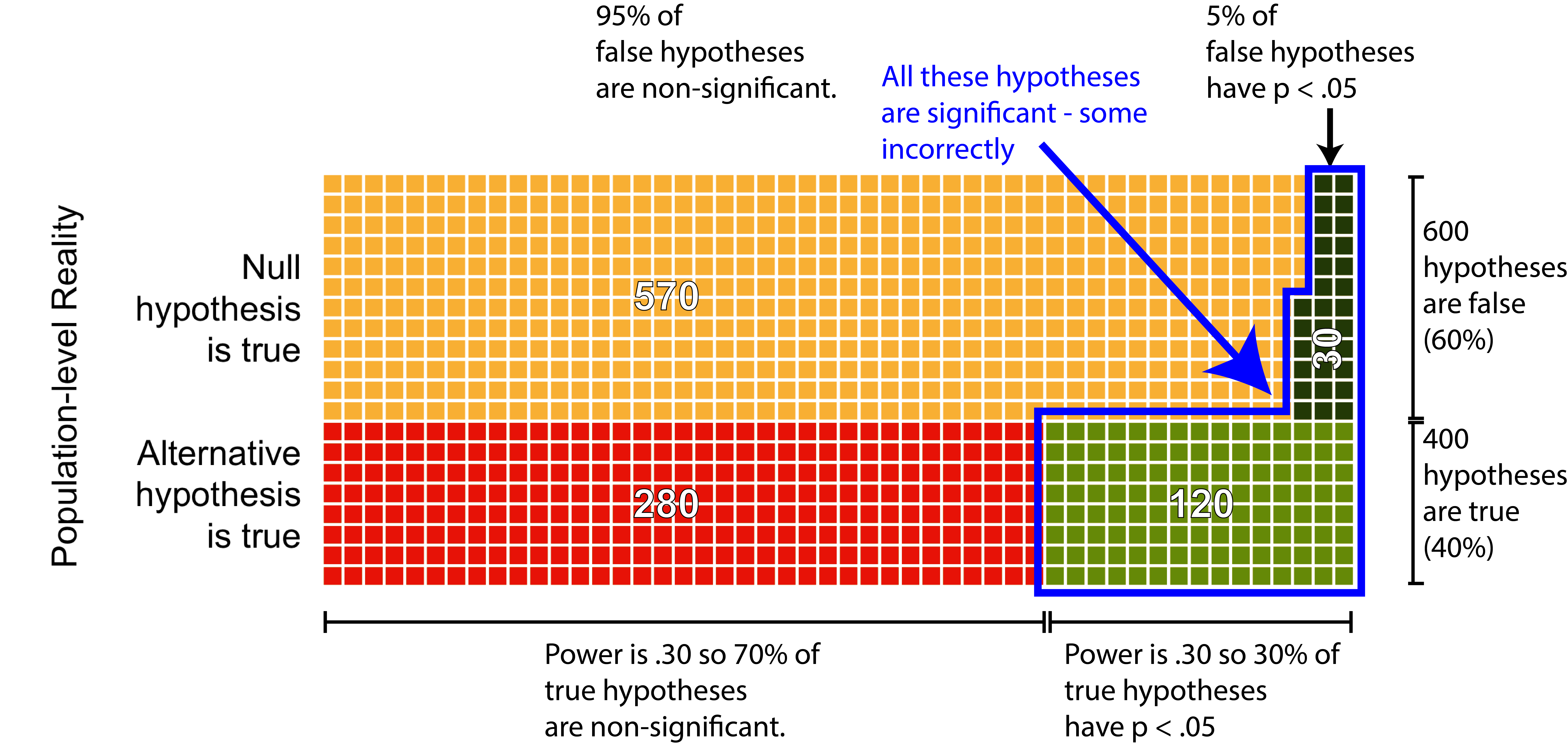
FIGURE 13.4: Illustrating there are two ways to obtain a significant effect.
As illustrated in Figure 13.5, below, the positive predictive value (PPV) is simply the proportion of statistically significant hypotheses that are true positives.
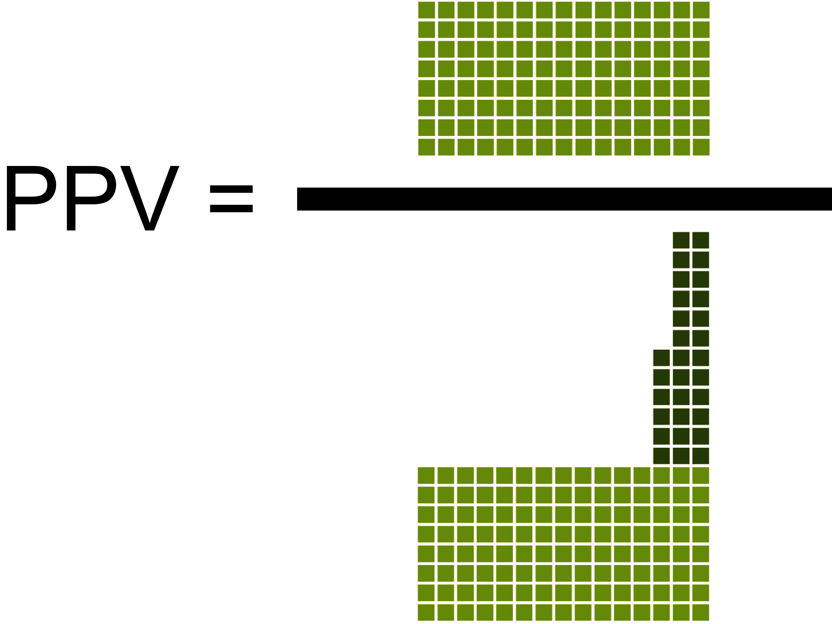
FIGURE 13.5: Graphical illustration of the PPV formula.
Placing numbers into the equation:
\[ \begin{aligned} PPV &= \frac{120 }{120 + 30} \\ &= \frac{120}{150} \\ &= 0.80 \end{aligned} \]
We see that the positive predictive value is .80 in this circumstance. That is, if we obtain a significant p-value there is an 80% chance there really is an effect.
13.4 Formal explanation
A more formal explanation of PPV can be made by thinking in terms of the area of square that is 1.0 units by 1.0 units. The length of each side corresponds a length of 1.0 because probabilities range from 0 to 1.0. Indeed, we can represent the probability of an hypothesis being true, P(effect), or false, P(no effect), along the right edge of the square. This is illustrated in Figure 13.6 below.
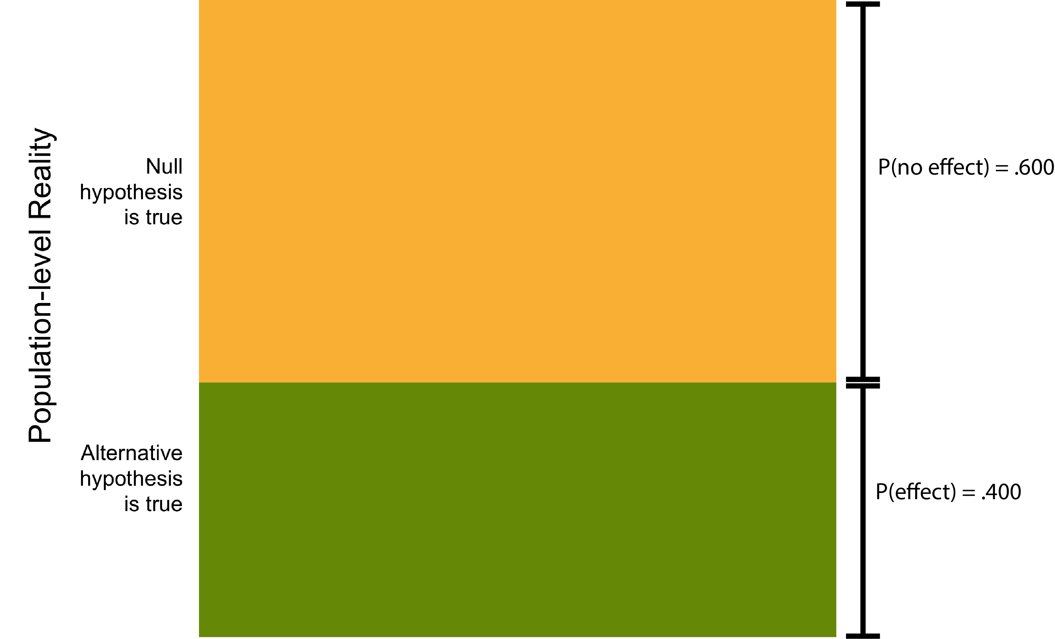
FIGURE 13.6: Representing probabilities on a square
13.4.1 No effect
Likewise, we can indicate the probability of a Type I Error on the diagram as well. Specifically, \(\alpha = .05\) is the distance, moving right to left, from the top right corner of the square. This is illustrated in Figure 13.7 below.
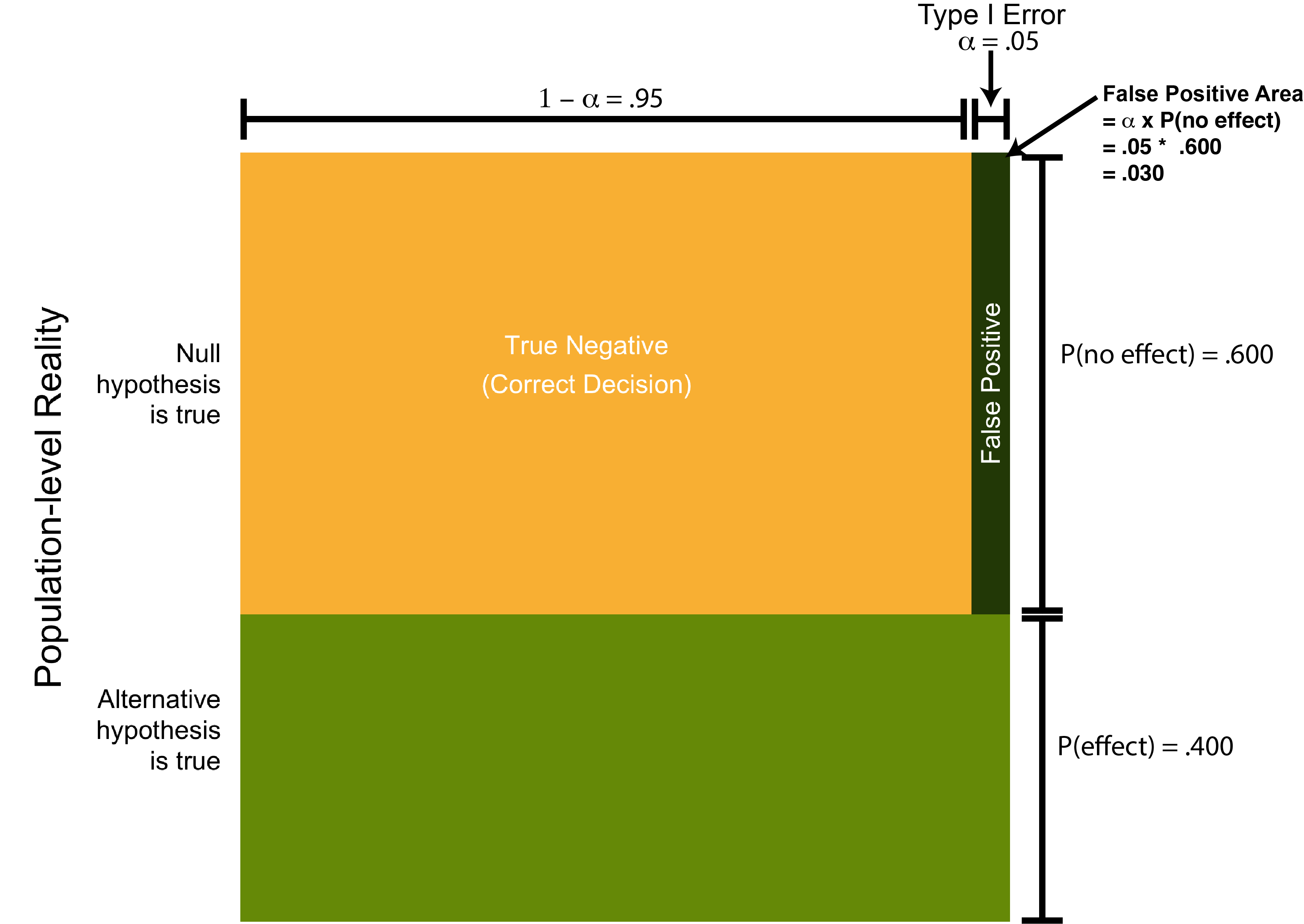
FIGURE 13.7: Representing Type I Error on the square
So far the probability of there being no effect, P(no effect), was indicated by a length (.600). Likewise, the probability of there being a Type I Error was indicated by a length (.05).
\[ \begin{aligned} P(\text{no effect}) &= 0.600 \\ P(\text{Type I Error}) &= 0.05 \\ \end{aligned} \]
We can use these together to determine the dark green area (nearly black area) on Figure 13.7 which represents the joint probability of there being no effect and obtaining a Type I Error. The \(\cap\) symbol indicates “and” which implies you need to multiply the two values.
You can see the probability .030 is similar to the count of 30 we had for this area in the informal explanation.
\[ \begin{aligned} P(\text{Type I Error} \cap \text{no effect} ) &= (\alpha) \cap P(\text{no effect}) \\ &= (.05)(.600) \\ &= 0.030 \end{aligned} \]
13.4.2 Effect
So far the probability of there being an effect, P(effect), was indicated by a length (.400). Likewise, the probability of finding that effect (i.e., power) can be indicated by a length (.30) as per Figure 13.8 below.
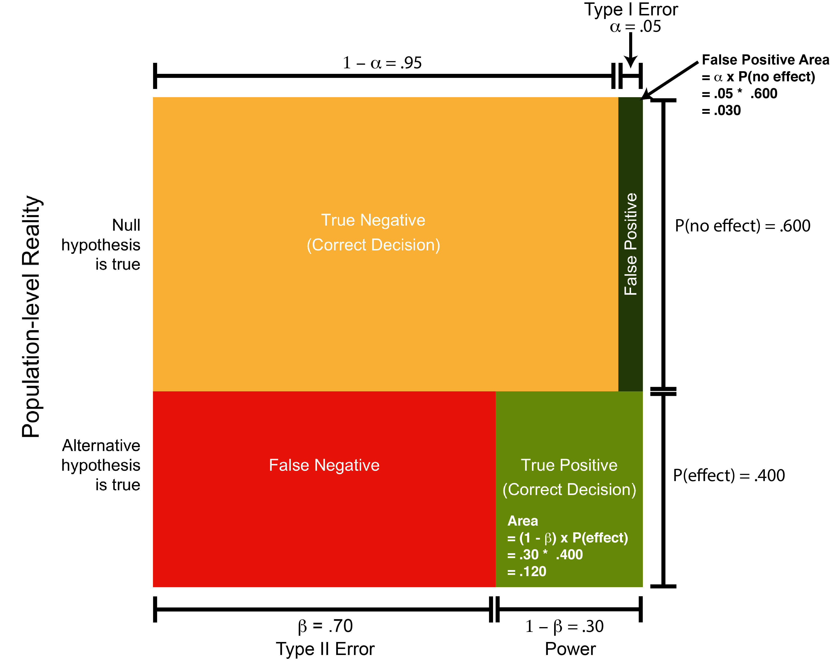
FIGURE 13.8: Representing power on the square
In this figure there are two important distances that represent probabilities as indicated below. Note that we often refer to power using the notation \(1 - \beta\).
\[ \begin{aligned} P(\text{effect}) &= 0.400 \\ (1 - \beta) &= 0.30 \\ \end{aligned} \]
We can use these together to determine the dark green area on the figure which represents the joint probability of there being an effect and obtaining a significant p-value. You can see the joint probability .030, below, is similar to the count of 30 we had for this area in the informal explanation.
\[ \begin{aligned} P(\text{power} \cap \text{effect}) &= (1 - \beta) \cap P(\text{effect})\\ &= (.30)(.400) \\ &= 0.120 \end{aligned} \]
13.4.3 Calculation
We can then calculate positive predictive value using the same logic as the informal case - but using formal equations. You can see in the equations below that some probabilities (.030, .120, and .150) correspond to the counts (30, 120, and 150) from the informal explanation above.
\[ \begin{aligned} PPV &= \frac{P(\text{effect} \cap \text{sig. p-value})}{P(\text{effect} \cap \text{sig. p-value}) + P(\text{no effect} \cap \text{sig. p-value})} \\ &= \frac{(1 - \beta)P(\text{effect})}{(1 - \beta)P(\text{effect}) + \alpha P(\text{no effect})}\\ &= \frac{(.30)(.400)}{(.30)(.400) + (.05)(.600)}\\ &= \frac{0.120}{0.120 + 0.030}\\ &= \frac{0.120}{0.150}\\ &= 0.80\\ \end{aligned} \]
Thus, the positive predictive value is .80. This indicates that if you obtain a significant p-value in your study there is an 80% chance there really is an effect.
13.4.4 Alternative calculation
You might also see positive predictive values expressed using an odds ratio (OR). This can create confusion - but it’s important to realize this alternative version of the formula is just an algebraic rearrangement. You can see this alternative version of the formula below and note that you obtain the same answer.
\[ \begin{aligned} PPV &= \frac{(1 - \beta)(OR)}{(1 - \beta)(OR) + \alpha}\\ &= \frac{(1 - \beta)(\frac{P(\text{effect})}{P(\text{no effect})})}{(1 - \beta)(\frac{P(\text{effect})}{P(\text{no effect})}) + \alpha}\\ &= \frac{(.30)(\frac{.400}{.600})}{(.30)(\frac{.400}{.600}) + \alpha}\\ &= \frac{(.30)(0.6666667)}{(.30)(0.6666667) + .05}\\ &= \frac{.20}{.20 + .05}\\ &= 0.80\\ \end{aligned} \]
13.4.5 Touchstone
You may, or may not, have noticed something familiar when we started working with the square as means of describing the numbers required for the positive predictive value calculation. Specifically, the square is very similar to the standard 2 x 2 table used to represents Type I Errors (false positives) and Type II Errors (false negatives). In Figure 13.9 I’ve placed a colour coded version of this table so that you can see the similarities with the calculation approach used above.
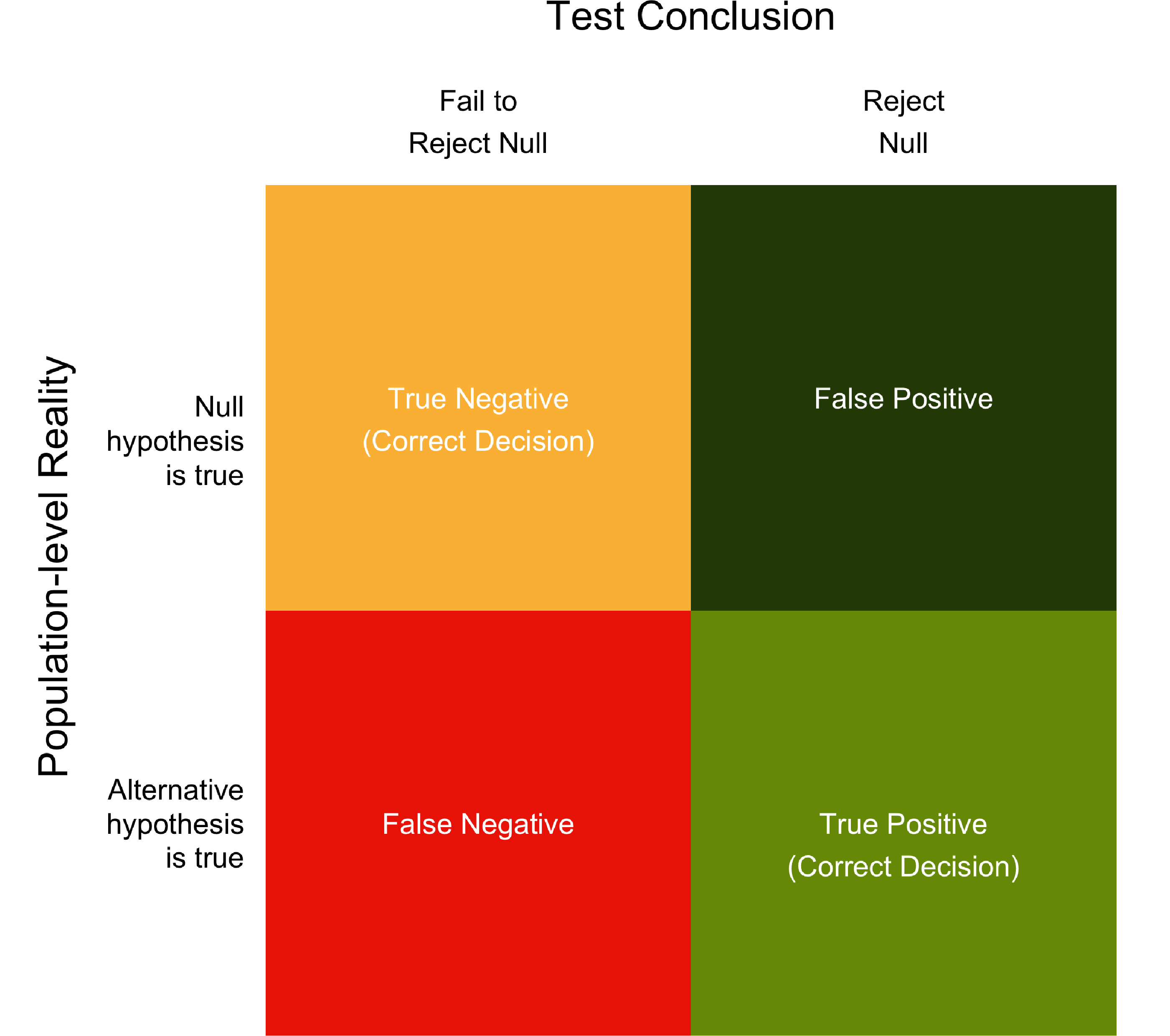
FIGURE 13.9: Table illustrating conclusion errors.
13.5 Calculating power for your study
Although we do a sample size analysis before collecting data - we are often unable to obtain the desired sample size. We can determine the consequences of failing to obtain the desired sample size by calculating positive predictive value. The first step in doing so is calculating the power for your study based on the number of participants you actually obtained.
To calculate the power for your study you need to use the same estimate of the population effect size that you used in original sample size analysis. You merely enter that same smallest effect size of interest (i.e., population level effect) and your obtained sample size into the R functions and it will return the power for your study - based on the sample size you actually obtained.
The examples below all illustrate a population-level effect (i.e., smallest effect size of interest from the original power analysis) and the obtained sample size. Check out the next section to see how to use this information to calculate the positive predictive value for your study.
13.5.1 Power independent groups \(t\)-test
library(pwr)
# Based on the previous study modify the settings below.
# For alternative: use "greater" for one-sided
# and "two.sided" for two-sided test
alternative <- "greater"
pop_d <- .24
sample_size_per_group <- 25

pwr_out <- pwr.t.test(d = pop_d,
                      n = sample_size_per_group,
                      type = "two.sample",
                      alternative = alternative)
Then we need to print our power / sample size analysis:
##
##      Two-sample t test power calculation
##
##               n = 25
##               d = 0.24
##       sig.level = 0.05
##           power = 0.2095
##     alternative = greater
##
## NOTE: n is number in *each* group
This analysis reveals that a) if we assume the population effect size is .24 (\(\delta = .24\)) and b) use a sample size of 25 per group, then our resulting power is 0.21. That is, if an effect exists, we have a 21% chance of finding it.
13.5.2 Power repeated measures \(t\)-test
library(pwr)
# Based on the previous study modify the settings below.
# For alternative: use "greater" for one-sided
# and "two.sided" for two-sided test
alternative <- "greater"
pop_d <- .17
n <- 30

pwr_out <- pwr.t.test(d = pop_d,
                      n = n,
                      type = "paired",
                      alternative = alternative)
Then we need to print our power / sample size analysis:
##
##      Paired t test power calculation
##
##               n = 30
##               d = 0.17
##       sig.level = 0.05
##           power = 0.2311
##     alternative = greater
##
## NOTE: n is number of *pairs*
This analysis reveals that a) if we assume the population effect size for our repeated measures \(t\)-test is 0.17 (\(\delta = 0.17\)) and b) we have a sample size of 30, then our resulting power is 0.23. That is, if an effect exists, we have a 23% chance of finding it.
13.5.3 Power correlations
library(pwr)
# Based on the previous study modify the settings below.
# For alternative: use "greater" for one-sided
# and "two.sided" for two-sided test
alternative <- "greater"
pop_r <- .18
n <- 100

pwr_out <- pwr.r.test(r = pop_r,
                      n = n,
                      alternative = alternative)
Then we need to print our power / sample size analysis:
##
##      approximate correlation power calculation (arctangh transformation)
##
##               n = 100
##               r = 0.18
##       sig.level = 0.05
##           power = 0.5623
##     alternative = greater
This analysis reveals that a) if we assume the population correlation is .18 (\(\rho = .18\)) and b) we use a sample size of 100, then our resulting power is 0.56. That is, if an effect exists, we have a 56% chance of finding it.
13.5.4 Equivalence independent t-test
13.6 Calculating PPV for your study
To calculate PPV for your study you simply use the previously presented formula for positive predictive value. Imagine that you conducted an independents groups t-test and determined your power was .21 you would calculate positive predictive value as below. You may assume the probability of your hypothesis being true is .400.
\[ \begin{aligned} PPV &= \frac{(1 - \beta)P(\text{effect})}{(1 - \beta)P(\text{effect}) + \alpha P(\text{no effect})}\\ &= \frac{(.21)(.400)}{(.21)(.400) + (.05)(.600)}\\ &= 0.74\\ \end{aligned} \]
Thus, if you obtained a significant p-value in this scenario there is only a 74% chance there really is an effect.