Chapter 9 From Script to Pipeline

At the end of Chapter 8 you had a complete, reproducible script that turned a raw Qualtrics file into clean analytic data. That script works. So why change anything?

This chapter answers that question and then shows you how to decompose your one long script into a small, organized project: a handful of short scripts, each doing one job, sitting in a sensible set of folders, all run by a single master script. This is a hands-on learning activity. You will build the project as you read, starting from the same data_qualtrics.csv file you already have. Nothing here is submitted or graded — the goal is for you to feel the difference between a 200-line script and a tidy pipeline in your own hands.

9.1 Required

This chapter rebuilds the Chapter 8 workflow as a structured project. You start from the data file you already have and build the project yourself by following along. A finished version is available as an “answer key” to check your work against — download it, but try to build the project yourself first.

Required Data
data_qualtrics.csv

Answer key (download, build it yourself first)
my-workflow-project.zip

The following CRAN packages must be installed. The last two (naniar and GGally) are new in this chapter; the rest you have already used.

Required CRAN Packages
apaTables
GGally
janitor
naniar
skimr
tidyverse

install.packages("naniar")
install.packages("GGally")

9.2 Why bother?

Before any mechanics, let us be honest about the cost: decomposing a working script into a project takes effort, and the script already runs. You deserve concrete reasons why the effort pays off. Here are five, and every one of them is true the moment you finish this chapter — no new tools required.

9.2.1 Find problems faster

This is the big one. Imagine there is a bug in your analysis — a scale is scored wrong, or a column got dropped that should not have been. In your Chapter 8 script, the problem could be anywhere in 200 lines. You scroll, you squint, you re-run the whole thing over and over, changing one line at a time, waiting for it to finish, looking again. The error is somewhere in the haystack and the whole haystack is one piece.

Now imagine the same work split into seven short scripts: import, clean, check missing data, score scales, apply exclusions, analyze. A scale scored wrong? That is stage 4. You open one short file, you see the whole stage at once, and you fix it. A bug in stage 4 of 7 means you look at stage 4. Small pieces localize errors — and they localize them for the most important debugger you have, which is you.

9.2.2 Get much better help from an AI assistant

You almost certainly use an AI assistant when you get stuck. Here is something most people learn the hard way: the quality of the help depends enormously on the size and clarity of what you paste in. Paste 200 lines of mixed-purpose code and ask “why is this wrong?” and the assistant has to guess what you even meant — the answer comes back vague and hedged. Paste one short, clearly named stage — “here is my 02-clean-recode.R, the recoded values look wrong” — and the assistant can see the entire unit: every input, every output, the one job it is supposed to do. The answer comes back sharp and specific.

Small, well-named pieces are not just easier for you to read. They are the unit an AI can actually reason about. Decomposing your script is, among other things, an investment in getting good answers for the rest of your career.

9.2.3 Read it again in six months

Code is read far more often than it is written, and the person who reads yours most is future-you. Six months from now, “the script” is an intimidating wall of text you have to re-understand from scratch. A folder of files named 01-import.R, 02-clean-recode.R, 03-missing-data.R is a table of contents. You know where things are before you open anything. The structure itself is documentation.

9.2.4 Reuse your work

Your “import a Qualtrics file” step and your “score the commitment scales” step are not single-use. The next study you run will need to import a Qualtrics file too. When that work lives in its own labelled stage rather than buried in the middle of a long script, you can lift it out and carry it to the next project. A pile of reusable parts is worth far more than one monolithic script.

9.2.5 Hand it off

Eventually someone else needs to run your analysis — a co-author, your supervisor, a labmate, a journal’s reproducibility checker. “Run 00-script-master.R” is an instruction anyone can follow. “Open this 200-line file and run it top to bottom, but watch out for the part in the middle where…” is not. A structured project with one obvious entry point is something you can actually give to another person.

You may have noticed two payoffs missing from this list: never re-running everything and never wondering whether a figure is stale. Those are real and powerful — but they are not honestly yours yet. A master script, which is what you build in this chapter, still re-runs every step every time. Earning those last two payoffs is what Chapter 10 is about. We will come back to them.

The throughline from Chapter 7 was begin with the end in mind and the promise of reproducibility. Decomposition is where that promise becomes personal and practical: a reproducible pipeline you can actually debug, reuse, and share.

9.3 One stage, one job

The core principle of decomposition is simple:

Each stage does one job, with explicit inputs and explicit outputs.

Look back at your Chapter 8 script with that principle in mind and the seams almost draw themselves. It already does a sequence of distinct jobs — import the file, clean and recode it, score the scales — it just does them all in one place. We are going to give each job its own file. Along the way we will also extend the pipeline with two stages the Chapter 8 script did not have but that any real analysis needs: a missing-data check and a participant-exclusion step. (This is why we kept the duration_in_seconds column back in Chapter 8 — the exclusions stage finally uses it.)

Here is the full set of stages we will build:

Script	The one job it does	Reads	Writes
01-import.R	Read the raw file, drop junk columns, make an ID	data-raw/data-qualtrics.csv	data-interim/01-imported.rds
02-clean-recode.R	Factors, Likert text → numbers, reverse-key	01-imported.rds	data-interim/02-cleaned.rds
03-missing-data.R	Diagnose missingness (reports + a figure)	02-cleaned.rds	files in output/
04-create-scales.R	Average items into scale scores	02-cleaned.rds	data-interim/03-scales-created.rds
05-exclusions.R	Drop participants per pre-registered rules	03-scales-created.rds	data-processed/analytic-data-final.rds
06-analysis-wrapper.R	Run the analysis, capture its output	(runs 07)	output/analysis-output.txt
07-analysis.R	Correlations, a table, a figure	analytic-data-final.rds	files in output/

A note on script names. In Chapter 7 we told you to name scripts beginning with script_ (for example script_qualtrics.R). That advice was for a project with one script. Once a project has several scripts that must run in a fixed order, numbering them — 01-import.R, 02-clean-recode.R, and so on — is simply the multi-script extension of that same habit: the number tells you (and your collaborators) the order to run them in, and the words after it tell you what each one does. Same spirit, more files.

Notice the input/output columns. Every stage reads a named file and writes a named file. That is what makes the stages independent: stage 4 does not care how stage 2 produced 02-cleaned.rds, only that the file exists. These .rds handoffs are the connective tissue of the whole project, and — as you will see in Chapter 10 — they are also the mental scaffolding for everything that follows.

Figure 9.1 is the same road map you first saw in Chapter 8, with two changes: the pipeline has grown the two new stages, and each box is now a file. The picture you used to navigate one long script has become the layout of an entire project.

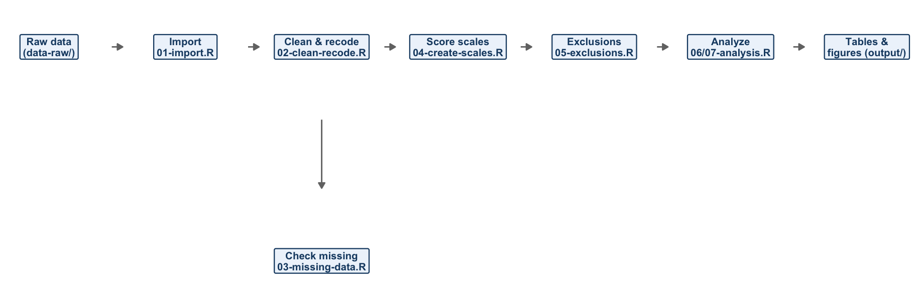
FIGURE 9.1: The road map, now as files. Each box is a numbered stage script; the missing-data check is a side branch that produces reports but does not change the data.

9.4 Project structure

Before we write any stage, we set up the folders. In RStudio, create a new project in an empty folder (File > New Project > New Directory > New Project). Inside it we will use four data-related folders, each with a clear role:

my-workflow-project/
├── data-raw/         <- the original data; NEVER edited
├── data-interim/     <- intermediate .rds files between stages
├── data-processed/   <- the finished analytic data set
├── output/           <- tables, figures, reports for humans
├── 01-import.R
├── 02-clean-recode.R
│   ... (the rest of the stages)
└── 00-script-master.R

This is the physical embodiment of the raw-versus-analytic-data distinction from Chapter 7. The flow runs strictly downhill: raw data comes in on the left, gets progressively more processed, and finished products for humans land in output/.

data-raw/ is sacred. The raw data file is the one thing in your project you can never reconstruct. Drop your data_qualtrics.csv into data-raw/ and then treat that folder as read-only: never edit those files by hand, never open them in Excel and re-save, never let a script write back into data-raw/. Every correction you need — a mislabeled value, a column to drop — happens in code, downstream. This is the single most important rule in the chapter, and it is what guarantees that your work can be reproduced from the original data.

Create the folder for raw data and drop your data file in it. We will let the master script create the other three folders automatically, so you do not have to.

9.5 Building the stages

Now we write the stages. We will go through them in order. Each one is a short script that reads its input, does its one job, and writes its output.

9.5.1 Stage 1 — Import

The first stage is your Chapter 8 loading code, lifted out and given a home. It reads the raw file, removes the Qualtrics columns you do not want, cleans the names, and creates a participant ID. The one new idea is the very last line: instead of leaving the result in memory, it saves the result to a file so the next stage can pick it up.

# Step 1: Import and Initial Setup

# Load Data ---------------------------------------------------------------
survey_file <- "data-raw/data-qualtrics.csv"

# Read header row for names
col_names <- names(read_csv(survey_file, n_max = 0, show_col_types = FALSE))

# Read data (skipping Qualtrics header rows 2 and 3)
raw_data <- read_csv(survey_file,
                     col_names = col_names,
                     skip = 3,
                     show_col_types = FALSE,
                     na = c("", "NA", "999")) # blanks, NA, and 999 are missing

# Select Columns ----------------------------------------------------------
cols_to_remove <- c("StartDate", "EndDate", "Status", "IPAddress", "Progress",
                    "Finished", "RecordedDate", "ResponseId", "RecipientLastName",
                    "RecipientFirstName", "RecipientEmail", "ExternalReference",
                    "LocationLatitude", "LocationLongitude", "DistributionChannel",
                    "UserLanguage")

analytic_data_survey <- raw_data |>
  select(!any_of(cols_to_remove)) |>
  clean_names() |>
  remove_empty("rows") |>
  remove_empty("cols")

# Create Participant ID ---------------------------------------------------
# Create the ID immediately so we can track rows even if the order changes
analytic_data_survey <- analytic_data_survey |>
  mutate(participant_id = row_number()) |>
  relocate(participant_id) # move it to the first column

# Save Interim File -------------------------------------------------------
# .rds preserves R's formatting (factor levels, types) — unlike .csv
write_rds(analytic_data_survey, "data-interim/01-imported.rds")

Two things to note. First, we read from data-raw/ and write to data-interim/ — the stage respects the folder structure. Second, we save with write_rds() rather than write_csv(). An .rds file stores the R object exactly as it is, including factor levels and column types, so the next stage gets back precisely what this stage produced.

Why this helps you: this single file is now the answer to “how did the raw data get loaded?” If the import ever looks wrong, this is the only file you need to read.

9.5.2 Stage 2 — Clean and recode

The second stage reads what the first stage wrote, converts sex to a factor, recodes the Likert text into numbers, and reverse-keys the reverse-worded items. This is the recoding work from Chapter 8, with one small upgrade we will point out.

# Step 2: Cleaning, Factors, and Recoding

# Load Previous Step ------------------------------------------------------
analytic_data_survey <- read_rds("data-interim/01-imported.rds")

# Factor Handling ---------------------------------------------------------
analytic_data_survey <- analytic_data_survey |>
  mutate(sex = as_factor(sex)) |>
  mutate(sex = fct_relevel(sex, "female", "intersex", "male"))

# Safety check: warn if an unexpected sex level shows up
expected_sex <- c("female", "intersex", "male")
unexpected <- setdiff(levels(analytic_data_survey$sex), expected_sex)
if (length(unexpected) > 0) {
  warning("Check Data! Unexpected sex levels found: ",
          paste(unexpected, collapse = ", "))
}

# Likert Recoding (text to numbers) ---------------------------------------
likert7_recode <- c(
  "Strongly Disagree" = 1, "Moderately Disagree" = 2, "Slightly Disagree" = 3,
  "Neither Agree nor Disagree" = 4, "Slightly Agree" = 5,
  "Moderately Agree" = 6, "Strongly Agree" = 7
)
likert5_recode <- c(
  "Strongly Disagree" = 1, "Disagree" = 2, "Neutral" = 3,
  "Agree" = 4, "Strongly Agree" = 5
)

analytic_data_survey <- analytic_data_survey |>
  mutate(across(.cols = contains("likert7"), .fns = ~ likert7_recode[.x])) |>
  mutate(across(.cols = contains("likert5"), .fns = ~ likert5_recode[.x]))

# Reverse Keying ----------------------------------------------------------
analytic_data_survey <- analytic_data_survey |>
  mutate(across(.cols = ends_with("_likert7rev"), .fns = ~ (7 + 1) - .x)) |>
  rename_with(.fn = ~ str_replace(.x, "_likert7rev", "_likert7"),
              .cols = ends_with("_likert7rev"))

# Save Interim File -------------------------------------------------------
write_rds(analytic_data_survey, "data-interim/02-cleaned.rds")

This stage uses the compact named lookup vector for the Likert recoding — the alternative we flagged in Chapter 8. It also adds a small safety check: if the sex column ever contains a level we did not expect (a typo like "mmale", say), the script issues a warning instead of silently sailing past it. Little checks like this are easy to add once a stage has a single, clear job.

9.5.3 Stage 3 — Missing-data diagnostics

This is a new stage, and it has a different shape from the others: it does not change the data. Instead it reads the cleaned data and produces three diagnostic products for you to look at — a report of which items have the most missing values, a list of participants who skipped a lot of the scale items, and a visual missingness map. Because it changes nothing, it writes its outputs to output/ and does not write an .rds file for the next stage. It is a side branch (look back at Figure 9.1).

# Step 3: Missing Data Evaluation

# Load Previous Step ------------------------------------------------------
analytic_data_survey <- read_rds("data-interim/02-cleaned.rds")

# Pull out just the scale items, which is what we want to screen
scale_items <- analytic_data_survey |>
  select(starts_with("aff_com"), starts_with("contin_com"),
         starts_with("norm_com"), starts_with("job_aff"))

# 1. Which items have the most missing data?
missing_summary <- scale_items |>
  miss_var_summary() |>   # from the naniar package
  filter(n_miss > 0)
print(missing_summary)
write_csv(missing_summary, "output/data-table-missing-by-item.csv")

# 2. Which participants are missing more than 20% of the scale items?
high_missing_participants <- analytic_data_survey |>
  rowwise() |>
  mutate(pct_missing = mean(is.na(c_across(c(
    starts_with("aff_com"), starts_with("contin_com"),
    starts_with("norm_com"), starts_with("job_aff"))))) * 100) |>
  ungroup() |>
  filter(pct_missing > 20) |>
  select(participant_id, pct_missing)
print(high_missing_participants)
write_csv(high_missing_participants, "output/data-table-missing-by-participant.csv")

# 3. A visual map of missingness (black = missing)
plot_missing <- vis_miss(scale_items) +
  labs(title = "Missing Data Map (Scale Items Only)")
ggsave("output/figure-missing-data-map.png", plot = plot_missing,
       width = 20, height = 20, dpi = "print")

The naniar package gives us miss_var_summary() and vis_miss() for free. The point of this stage is to look before you leap: you want to know about a participant who skipped half the survey before you average their answers into a scale score.

9.5.4 Stage 4 — Create scale scores

This stage reads the cleaned data (not the missing-data stage — remember, that stage was a side branch) and averages the items into the four commitment and job-satisfaction scale scores, then drops the now-redundant item columns.

# Step 4: Scale Creation

# Load Previous Step ------------------------------------------------------
analytic_data_survey <- read_rds("data-interim/02-cleaned.rds")

# Create Scale Scores -----------------------------------------------------
analytic_data_survey <- analytic_data_survey |>
  rowwise() |>
  mutate(
    affective_commitment   = mean(c_across(starts_with("aff_com")),    na.rm = TRUE),
    continuance_commitment = mean(c_across(starts_with("contin_com")), na.rm = TRUE),
    normative_commitment   = mean(c_across(starts_with("norm_com")),   na.rm = TRUE),
    job_satisfaction       = mean(c_across(starts_with("job_aff")),    na.rm = TRUE)
  ) |>
  ungroup()    # always ungroup after rowwise()!

# Drop the item columns now that the scale scores exist
analytic_data_survey <- analytic_data_survey |>
  select(-starts_with("aff_com"), -starts_with("contin_com"),
         -starts_with("norm_com"), -starts_with("job_aff"))

# Save Interim File -------------------------------------------------------
write_rds(analytic_data_survey, "data-interim/03-scales-created.rds")

9.5.5 Stage 5 — Exclusions

Now the duration_in_seconds column earns its keep. This stage applies the participant-exclusion rule — here, dropping anyone who finished the survey implausibly fast (under two minutes). It reads the scored data and writes the final analytic data set into data-processed/.

# Step 5: Exclusions
# Exclusion rules should be decided in advance (ideally pre-registered).
# Here we drop participants who finished in under 2 minutes (120 seconds).

# Load Previous Step ------------------------------------------------------
analytic_data_survey <- read_rds("data-interim/03-scales-created.rds")

# Exclusions --------------------------------------------------------------
initial_n <- nrow(analytic_data_survey)

analytic_data_survey <- analytic_data_survey |>
  filter(duration_in_seconds >= 120)

final_n <- nrow(analytic_data_survey)
message(paste("Dropped", initial_n - final_n, "participants due to speed checks."))

# Final Save --------------------------------------------------------------
write_rds(analytic_data_survey, "data-processed/analytic-data-final.rds")

glimpse(analytic_data_survey)

Notice this stage’s output lands in data-processed/, not data-interim/. The folder names tell the story: data-interim/ holds work in progress; data-processed/ holds the finished, analysis-ready data set.

Exclusion decisions change your results, so they should never be made casually or after you have seen how they affect your findings. Decide your exclusion rules in advance — ideally as part of a pre-registration (Chapter ??). Putting exclusions in their own clearly named stage has a side benefit: anyone reading your project can see exactly who was dropped and why.

9.5.6 Stages 6 and 7 — Analysis

The last two stages run the analysis. We split them in two for a practical reason. 07-analysis.R does the actual statistics — descriptive statistics, a correlation table, and a scatterplot matrix. 06-analysis-wrapper.R is a tiny wrapper whose only job is to run the analysis script and capture everything it prints into a text file, so you have a permanent record of the console output.

# Step 6: Analysis Wrapper
# Runs the analysis script and captures its console output to a text file.
capture.output(
  source("07-analysis.R", echo = TRUE),
  file = "output/analysis-output.txt"
)

# Step 7: Analysis

# Start clean and set a seed so any randomness (e.g. jitter) is reproducible
rm(list = ls())
set.seed(12345)

library(tidyverse)
library(GGally)
library(skimr)
library(apaTables)

# Load Previous Step ------------------------------------------------------
analytic_data_survey <- read_rds("data-processed/analytic-data-final.rds")

# Analysis ----------------------------------------------------------------
skim(analytic_data_survey)

# Descriptive statistics + correlations among the commitment scales
data_plot <- analytic_data_survey |>
  select(contains("commitment"))

apa.cor.table(data_plot,
              filename = "output/table-correlation-descriptive-statistics.doc",
              table.number = 1)

# A scatterplot matrix of the commitment scales
cor_plot <- ggpairs(data_plot,
                    upper = "blank",
                    lower = list(continuous = wrap("points", alpha = 0.3)),
                    diag  = list(continuous = wrap("barDiag", bins = 15,
                                                   color = "black", fill = "black"))) +
  theme_linedraw(10)

ggsave("output/figure-pairs-plot.png", plot = cor_plot,
       width = 7, height = 7, units = "in", dpi = 300)

print(cor_plot)

The analysis stage produces real deliverables in output/: an APA-formatted correlation table you can drop into a manuscript and a publication-quality figure.

9.6 The master script

You now have seven stage scripts. The last piece ties them together: a single master script that runs them all, in order, from a clean slate. This is the project’s front door — the one file a collaborator (or future-you) runs to reproduce everything.

# Date: 2026-01-15 (Use YYYY-MM-DD format)
# Name: [Your Name]
# Purpose: Master — runs all data-preparation steps in order

# 1. Setup Environment ----------------------------------------------------
library(tidyverse)
library(janitor)
library(skimr)
library(naniar)   # for missing-data visualization

# Clear memory to ensure a clean, reproducible run
rm(list = ls())

# Create the working folders if they do not already exist
if (!dir.exists("data-interim"))   dir.create("data-interim")
if (!dir.exists("data-processed")) dir.create("data-processed")
if (!dir.exists("output"))         dir.create("output")

# 2. Execute Pipeline -----------------------------------------------------
message("--- Running Step 1: Import ---")
source("01-import.R", echo = TRUE)

message("--- Running Step 2: Cleaning ---")
source("02-clean-recode.R", echo = TRUE)

message("--- Running Step 3: Evaluate missing data ---")
source("03-missing-data.R", echo = TRUE)

message("--- Running Step 4: Create scales ---")
source("04-create-scales.R", echo = TRUE)

message("--- Running Step 5: Excluding participants ---")
source("05-exclusions.R", echo = TRUE)

message("--- Running Step 6: Analysis and Visualization ---")
source("06-analysis-wrapper.R", echo = TRUE)

message("--- Pipeline Complete! ---")

Read the master script top to bottom and you have the entire project in one glance. It loads the packages every stage needs, clears memory so the run does not depend on whatever happened to be sitting in your session, makes sure the output folders exist, and then source()s each stage in order. To reproduce the whole analysis from raw data, you do one thing: open the project and run 00-script-master.R.

The master script loads the shared packages once, at the top. That is why the individual stage scripts do not each call library(tidyverse) — they inherit the packages the master script already loaded. (The analysis stage is the one exception: because the wrapper runs it with a cleared memory, it loads its own packages.)

9.6.1 The handoffs make the dependencies visible

Step back and look at what the .rds files are doing. Stage 1 writes 01-imported.rds; stage 2 reads it. Stage 2 writes 02-cleaned.rds; stages 3 and 4 both read it. Those read/write pairs are the dependencies of your pipeline, written down in plain sight. You can trace any product back to its source by following the files: the pairs plot came from the final analytic data, which came from the scored data, which came from the cleaned data, which came from the import, which came from the raw file.

Hold onto this idea. Right now you are the one keeping track of which file feeds which — by reading the master script and remembering the order. In Chapter 10 we hand that bookkeeping to a tool, and these visible handoffs are exactly what makes the handover possible.

9.7 Where even this strains

Take stock of what you have. Your one long script is now a structured project: sacred raw data, numbered single-purpose stages, visible handoffs between them, finished products collected in output/, and a single master script that reproduces everything from scratch. This is a genuine, shareable, reproducible workflow. It is the floor every research project should reach, and most never do. This is the win of the chapter — do not undersell it.

And yet. Run the master script and three honest limitations show up:

1. It re-runs everything, every time. Change one line in the analysis stage and 00-script-master.R dutifully re-imports the raw file, re-cleans it, re-scores the scales, and re-checks missing data — all unchanged — before finally reaching your edit. For this small project that is a few seconds. For a project with a slow step (big data, a simulation, a meta-analysis over thousands of studies) it is the difference between seconds and an hour.

2. You maintain the order and the filenames by hand. The master script works because you listed the stages in the right order and you kept the write_rds() in one stage matching the read_rds() in the next. Rename a file or reorder two stages and nothing warns you — it just breaks, or worse, silently uses a stale file.

3. Staleness is invisible. Nothing in this project knows whether output/figure-pairs-plot.png is up to date with the current data-raw/. If you edit the raw data but forget to re-run, the old figure sits there looking perfectly fine. You cannot tell, by looking, what is current and what is stale.

These are not flaws in your work — your project is correct. They are the limits of any master-script approach. What if a tool could maintain the order for you, re-run only the stages affected by a change, and tell you at a glance exactly what is up to date and what is stale?

That tool exists, it is built for R, and it is the subject of the next chapter.

What you built (follow-along). You decomposed your Chapter 8 Qualtrics script into a structured project: a sacred data-raw/ folder, numbered single-purpose stage scripts with visible .rds handoffs, an output/ folder of finished products, and a master script that runs the whole pipeline end to end. Compare your work against the my-workflow-project.zip answer key. Nothing is submitted.