Chapter 10 Orchestrating with targets
At the end of Chapter 9 you had a real, reproducible project: numbered stages, a sacred data-raw/ folder, and a master script that runs everything from raw data to finished figures. You also had three honest complaints — it re-runs everything every time, you maintain the order and filenames by hand, and you cannot tell what is stale.
This chapter introduces a tool that fixes all three: the targets package. We will take the project you built in Chapter 9 and orchestrate it — turn it from a list of scripts you run in order into a pipeline a tool runs for you, intelligently. As before, this is a hands-on, follow-along build. Nothing is submitted.
10.1 Required
You will convert the Chapter 9 project into a targets pipeline by following along. A finished version is available as an answer key — build it yourself first, then compare.
| Required Data |
|---|
| data_qualtrics.csv |
| Answer key (download, build it yourself first) |
|---|
| my-workflow-project-targets.zip |
The one new package is targets. You will also use naniar, GGally, and apaTables from the previous chapter.
| Required CRAN Packages |
|---|
| apaTables |
| GGally |
| janitor |
| naniar |
| targets |
| tidyverse |
10.2 Why go further?
Your Chapter 9 project is good. Reaching for another tool needs to clear a real bar, so here are the payoffs — and unlike the last chapter, these are exactly the ones a master script cannot give you.
10.2.1 Stop re-running everything
This is the headline. With a master script, changing one line in the analysis stage re-runs the entire pipeline from the raw file down. targets watches what actually changed and re-runs only the parts affected by that change, skipping everything else because it can prove those parts are unaffected. Edit the analysis and targets reruns the analysis — it does not re-import the CSV or recompute the scales.
On this small example the saving is a few seconds. But picture the project this course is really preparing you for: a meta-analysis over thousands of studies, where computing effect sizes takes an hour. Change the final figure and a master script makes you wait an hour to re-run work that did not change. targets makes you wait for the figure. That is the difference between a tool you fight and a tool that works for you.
10.2.2 Pick up after a crash
A long master script that dies in stage 6 leaves you nowhere — you fix the problem and start again from stage 1. Because targets stores each completed stage, a rerun picks up from the last good stage instead of from zero. Your expensive early steps are banked.
10.2.3 Never wonder whether a number is stale
This is the one that protects your credibility. With a master script you can never be sure that figure-pairs-plot.png reflects the current data — maybe you edited the raw file and forgot to re-run. targets tracks this for you and shows it at a glance: it knows which targets are up to date and which are stale, and it will not let a stale result masquerade as current. You stop wondering whether a figure in your manuscript matches your data, because the tool guarantees it.
Recall the three complaints that ended Chapter 9: re-runs everything, hand-maintained order, invisible staleness. Hold them in mind as a checklist — by the end of this chapter targets will have answered all three. The question driving the chapter is: what if a tool maintained the order for you and re-ran only what changed?
10.3 On-ramp: turning a script into a function
Before we can use targets, we need one new skill. targets does not run loose scripts; it runs functions. So our first job is to learn to turn a stage script into a function. If you have never written a function, this section is the gentle on-ramp.
A function is a named recipe: you give it some ingredients (its arguments), it does its work, and it hands back one result (with return(), or simply as the last value it computes). The shape is always the same:
my_function <- function(ingredient1, ingredient2) {
  # ... do some work using the ingredients ...
  return(result)   # hand back exactly one object
}
Let us convert the import stage. Here is the before — the relevant part of 01-import.R from Chapter 9. Notice how it reads from a hard-coded filename at the top and writes to a hard-coded file at the bottom:
# BEFORE: a script
survey_file <- "data-raw/data-qualtrics.csv"          # hard-coded input

col_names <- names(read_csv(survey_file, n_max = 0, show_col_types = FALSE))
raw_data  <- read_csv(survey_file, col_names = col_names, skip = 3,
                      show_col_types = FALSE, na = c("", "NA", "999"))
# ... drop junk columns, clean names, make an ID ...

write_rds(analytic_data_survey, "data-interim/01-imported.rds")   # hard-coded output
And here is the after — the same logic as a function. The input filename becomes an argument (survey_file), and instead of writing a file at the end, the function return()s the data object:
# AFTER: a function
import_survey <- function(survey_file) {
  col_names <- names(readr::read_csv(survey_file, n_max = 0, show_col_types = FALSE))

  raw_data <- readr::read_csv(
    survey_file, col_names = col_names, skip = 3,
    show_col_types = FALSE, na = c("", "NA", "999")
  )

  cols_to_remove <- c(
    "StartDate", "EndDate", "Status", "IPAddress", "Progress",
    "Finished", "RecordedDate", "ResponseId", "RecipientLastName",
    "RecipientFirstName", "RecipientEmail", "ExternalReference",
    "LocationLatitude", "LocationLongitude", "DistributionChannel",
    "UserLanguage"
  )

  analytic_data_survey <- raw_data |>
    select(!any_of(cols_to_remove)) |>
    clean_names() |>
    remove_empty("rows") |>
    remove_empty("cols")

  # The last expression is what the function returns
  analytic_data_survey |>
    mutate(participant_id = row_number()) |>
    relocate(participant_id)
}
Three changes turned the script into a function, and they are the same three changes every time:
- Inputs become arguments. The hard-coded
"data-raw/data-qualtrics.csv"is gone; the function takessurvey_fileas an argument, so it can import any file you point it at. - The output is returned, not written. No
write_rds(). The function hands back the data object. Whoever calls the function decides what to do with it — and as you will see,targetswill store it for us automatically. - One job, one returned object. A target tracks exactly one output, so a function for
targetsdoes one job and returns one thing.
targets needs — it is exactly the unit you can hand to an AI assistant for precise help. “Here is my import_survey() function; the participant IDs come out wrong” gives the assistant a complete, self-contained problem it can fully reason about. The same property that makes a function trackable by targets makes it legible to an AI — and to your future self.
We will write the rest of the pipeline’s functions the same way. For now, just absorb the move: inputs in as arguments, one object out via the return.
10.4 The DAG idea — draw it first
We have been using a road map of the pipeline since Chapter 8 without giving it a technical name. It is time to name it. That picture — boxes connected by arrows showing what feeds what — is a DAG: a Directed Acyclic Graph. Break the term apart:
- Graph — boxes (called nodes) connected by arrows (called edges). Here each node is a step of your pipeline (or its output) and each edge is a dependency.
- Directed — the arrows have a direction. “clean → scales” means scoring the scales depends on the cleaning. The arrow points the way the data flows.
- Acyclic — no loops. You cannot have A depend on B which depends on A. This is what makes the pipeline runnable: there is always a valid order in which every step runs only after the steps it needs are finished.
That is the whole concept. You have understood the idea since Chapter 8; the only new thing is the vocabulary.
A DAG gives a tool two superpowers. First, correct order for free: it reads the graph and figures out the order to run things, so you never sequence stages by hand again. Second, and this is the one that matters most, skip what is unchanged: it tracks each node’s inputs, and if a node’s inputs and code are untouched, it skips that node and everything downstream that is still valid — re-running only the part of the graph your change actually affected.
The most transferable habit in this entire book is this: before you write pipeline code, sketch the DAG. On paper, or on a whiteboard, draw a box for each step and an arrow for each “this feeds that.” For our project the sketch is Figure 10.1 — the same road map from Chapter 9, which we are about to watch the computer draw for itself.
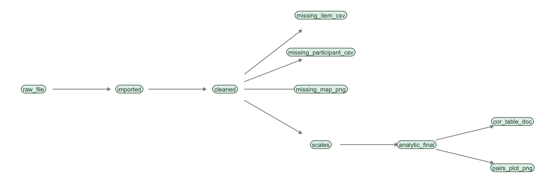
FIGURE 10.1: The pipeline sketched as a DAG. cleaned feeds three missing-data diagnostics, and also feeds scales; analytic_final feeds the two analysis deliverables. These are the node names we will use in the code.
Keep this sketch beside you. In a moment targets will draw its own version of it, and the satisfying payoff is that the two will match.
10.5 Building _targets.R incrementally
A targets project has a particular layout, and it is close to what you already built:
my-workflow-project-targets/
├── data-raw/
│   └── data-qualtrics.csv
├── R/
│   └── functions.R     <- all your stage functions live here
├── output/             <- file deliverables (.csv, .png, .doc)
└── _targets.R          <- defines the pipeline (the DAG)
Two files do the work. R/functions.R holds the functions (the import_survey()-style recipes from the on-ramp). _targets.R is the pipeline definition: it lists the targets and, by referring to them by name, tells targets how they connect. We will build _targets.R one target at a time and watch the DAG grow.
10.5.1 Start with the raw file and the import
Create _targets.R with just enough to import the data. A targets pipeline is a list() of tar_target() calls; each tar_target(name, expression) says “make a target called name by running expression.”
# _targets.R  (first version)
library(targets)

tar_option_set(packages = c("tidyverse", "janitor"))
tar_source("R/functions.R")   # load our functions

list(
  tar_target(raw_file, "data-raw/data-qualtrics.csv", format = "file"),
  tar_target(imported, import_survey(raw_file))
)library(tidyverse). In a targets project the packages are declared once, in tar_option_set(packages = ...), not with library() calls scattered through your functions. targets makes those packages available to every target. This is the kind of bookkeeping the tool now does for you.
Two details earn their keep here. format = "file" tells targets that raw_file is a file on disk: it watches the file’s contents, so if you ever edit data-raw/data-qualtrics.csv, targets knows the whole pipeline is now stale. And notice that imported is built by calling import_survey(raw_file) — targets sees that imported uses raw_file, and from that single fact it infers the arrow raw_file → imported. You never declare the order; it is read from the code.
Now build it. From the project, run:
▶ dispatched target raw_file
● completed target raw_file [0.001 seconds]
▶ dispatched target imported
● completed target imported [0.4 seconds]
▶ ended pipeline [0.5 seconds]
And draw what you have:
Two nodes, one arrow. The computer just drew the left end of your road map.
10.5.2 Add the next stage, and the next
Now grow the pipeline. Add the cleaning step — and again, all you do is refer to the previous target by name:
list(
  tar_target(raw_file, "data-raw/data-qualtrics.csv", format = "file"),
  tar_target(imported, import_survey(raw_file)),
  tar_target(cleaned,  clean_recode(imported))     # <- new
)
Run tar_make() again and watch what happens:
✔ skipped target raw_file
✔ skipped target imported
▶ dispatched target cleaned
● completed target cleaned [0.3 seconds]
▶ ended pipeline [0.4 seconds]
Look carefully: raw_file and imported say skipped. targets already has them, nothing they depend on changed, so it does not redo them — it builds only the new cleaned target. You are seeing the central superpower in miniature. Call tar_visnetwork() again and the graph has grown a node.
You continue this way, adding one target per stage, calling tar_make() and tar_visnetwork() as you go, watching the graph grow and only the new nodes build. Here is the complete _targets.R once every stage is in:
# _targets.R  (complete)
library(targets)

if (!dir.exists("output")) dir.create("output")

tar_option_set(
  packages = c("tidyverse", "janitor", "naniar", "GGally", "apaTables")
)
tar_source("R/functions.R")

list(
  # Source data — format = "file" tracks the file's contents
  tar_target(raw_file, "data-raw/data-qualtrics.csv", format = "file"),

  # Step 1: Import
  tar_target(imported, import_survey(raw_file)),

  # Step 2: Clean and recode
  tar_target(cleaned, clean_recode(imported)),

  # Step 3: Missing-data diagnostics (terminal; data unchanged)
  tar_target(missing_item_csv,
             write_missing_by_item(cleaned, "output/data-table-missing-by-item.csv"),
             format = "file"),
  tar_target(missing_participant_csv,
             write_missing_by_participant(cleaned, "output/data-table-missing-by-participant.csv"),
             format = "file"),
  tar_target(missing_map_png,
             save_missing_map(cleaned, "output/figure-missing-data-map.png"),
             format = "file"),

  # Step 4: Create scale scores
  tar_target(scales, create_scales(cleaned)),

  # Step 5: Apply exclusions
  tar_target(analytic_final, apply_exclusions(scales)),

  # Step 7: Analysis deliverables
  tar_target(cor_table_doc,
             save_cor_table(analytic_final, "output/table-correlation-descriptive-statistics.doc"),
             format = "file"),
  tar_target(pairs_plot_png,
             save_pairs_plot(analytic_final, "output/figure-pairs-plot.png"),
             format = "file")
)
Compare this list to your DAG sketch in Figure 10.1: every node is there, and every arrow is implied by which targets each expression mentions. cleaned is mentioned by the three missing-data targets and by scales, which is exactly the fan-out you drew.
10.5.3 The functions behind the targets
The pipeline above is short because the real work lives in R/functions.R. We wrote import_survey() together in the on-ramp; we write clean_recode() and create_scales() the same way — inputs in as arguments, one object returned. Here they are:
clean_recode <- function(analytic_data_survey) {
  analytic_data_survey <- analytic_data_survey |>
    mutate(sex = as_factor(sex)) |>
    mutate(sex = fct_relevel(sex, "female", "intersex", "male"))

  expected_sex <- c("female", "intersex", "male")
  unexpected <- setdiff(levels(analytic_data_survey$sex), expected_sex)
  if (length(unexpected) > 0) {
    warning("Check Data! Unexpected sex levels found: ",
            paste(unexpected, collapse = ", "))
  }

  likert7_recode <- c(
    "Strongly Disagree" = 1, "Moderately Disagree" = 2, "Slightly Disagree" = 3,
    "Neither Agree nor Disagree" = 4, "Slightly Agree" = 5,
    "Moderately Agree" = 6, "Strongly Agree" = 7
  )
  likert5_recode <- c(
    "Strongly Disagree" = 1, "Disagree" = 2, "Neutral" = 3,
    "Agree" = 4, "Strongly Agree" = 5
  )

  analytic_data_survey <- analytic_data_survey |>
    mutate(across(.cols = contains("likert7"), .fns = ~ likert7_recode[.x])) |>
    mutate(across(.cols = contains("likert5"), .fns = ~ likert5_recode[.x]))

  analytic_data_survey |>
    mutate(across(.cols = ends_with("_likert7rev"), .fns = ~ (7 + 1) - .x)) |>
    rename_with(.fn = ~ str_replace(.x, "_likert7rev", "_likert7"),
                .cols = ends_with("_likert7rev"))
}

create_scales <- function(analytic_data_survey) {
  analytic_data_survey |>
    rowwise() |>
    mutate(
      affective_commitment   = mean(c_across(starts_with("aff_com")),    na.rm = TRUE),
      continuance_commitment = mean(c_across(starts_with("contin_com")), na.rm = TRUE),
      normative_commitment   = mean(c_across(starts_with("norm_com")),   na.rm = TRUE),
      job_satisfaction       = mean(c_across(starts_with("job_aff")),    na.rm = TRUE)
    ) |>
    ungroup() |>
    select(-starts_with("aff_com"), -starts_with("contin_com"),
           -starts_with("norm_com"), -starts_with("job_aff"))
}
The chapter provides the remaining functions for you to study and reuse — they are the same logic from Chapter 9, wrapped as functions. The missing-data and analysis stages each write a file, so their functions take a path argument and return that path — that is the trick that lets a format = "file" target track the output file:
select_scale_items <- function(data) {
  data |>
    select(starts_with("aff_com"), starts_with("contin_com"),
           starts_with("norm_com"), starts_with("job_aff"))
}

write_missing_by_item <- function(data, path) {
  missing_summary <- select_scale_items(data) |>
    naniar::miss_var_summary() |>
    filter(n_miss > 0)
  readr::write_csv(missing_summary, path)
  path                       # return the path so targets can track the file
}

write_missing_by_participant <- function(data, path) {
  high_missing_participants <- data |>
    rowwise() |>
    mutate(pct_missing = mean(is.na(c_across(c(
      starts_with("aff_com"), starts_with("contin_com"),
      starts_with("norm_com"), starts_with("job_aff"))))) * 100) |>
    ungroup() |>
    filter(pct_missing > 20) |>
    select(participant_id, pct_missing)
  readr::write_csv(high_missing_participants, path)
  path
}

save_missing_map <- function(data, path) {
  plot_missing <- naniar::vis_miss(select_scale_items(data)) +
    labs(title = "Missing Data Map (Scale Items Only)")
  ggsave(path, plot = plot_missing, width = 20, height = 20, dpi = "print")
  path
}

apply_exclusions <- function(analytic_data_survey) {
  initial_n <- nrow(analytic_data_survey)
  analytic_data_survey <- analytic_data_survey |>
    filter(duration_in_seconds >= 120)
  final_n <- nrow(analytic_data_survey)
  message(paste("Dropped", initial_n - final_n, "participants due to speed checks."))
  analytic_data_survey
}

save_cor_table <- function(analytic_final, path) {
  commitment_data <- analytic_final |> select(contains("commitment"))
  apaTables::apa.cor.table(commitment_data, filename = path, table.number = 1)
  path
}

save_pairs_plot <- function(analytic_final, path) {
  set.seed(12345)
  commitment_data <- analytic_final |> select(contains("commitment"))
  cor_plot <- GGally::ggpairs(
    commitment_data,
    upper = "blank",
    lower = list(continuous = GGally::wrap("points", alpha = 0.3)),
    diag  = list(continuous = GGally::wrap("barDiag", bins = 15,
                                           color = "black", fill = "black"))
  ) + theme_linedraw(10)
  ggsave(path, plot = cor_plot, width = 7, height = 7, units = "in", dpi = 300)
  path
}
Notice what disappeared in the move to targets. There is no master script and no manual ordering — _targets.R plus the inferred DAG replace 00-script-master.R. There are no .rds handoffs and no data-interim/ folder — targets caches each target’s value for you under a hidden _targets/ folder, so the read_rds()/write_rds() pairs that connected your stages are gone. And there is no analysis wrapper to capture console output — targets records each target’s output itself.
10.5.4 The computer draws your map
Now the payoff promised in the DAG section. With the complete pipeline in place, ask targets to draw the graph. The figure below is generated live, while this book is being built — it is not a screenshot. (In the interactive HTML version you can drag the nodes around.)
Compare this to your hand sketch in Figure 10.1. It is the same graph — the map you have been navigating since Chapter 8, now drawn for you by the computer and, crucially, kept current automatically. That is the whole arc of the road map paying off: concept (Chapter 7) → road map of your script (Chapter 8) → road map as files (Chapter 9) → a live, machine-maintained DAG.
10.6 The payoff
Let us make the three promised payoffs concrete by actually using the built pipeline.
Pull any result into your session. You do not re-run anything to inspect a result; you read it from the cache with tar_read(). Here is the real final analytic data set, read live from the example pipeline:
## # A tibble: 129 × 8
##    participant_id duration_in_seconds year_of_birth sex
##             <int>               <dbl>         <dbl> <fct>
##  1              1                 244          1961 female
##  2              2                 134          2006 female
##  3              3                 237          2008 female
##  4              5                 151          1953 intersex
##  5              7                 393          1998 intersex
##  6              8                 165          1970 male
##  7              9                 315          1983 female
##  8             10                 262          1959 female
##  9             11                 370          2008 intersex
## 10             12                 200          1982 male
## # ℹ 119 more rows
## # ℹ 4 more variables: affective_commitment <dbl>,
## #   continuance_commitment <dbl>,
## #   normative_commitment <dbl>, job_satisfaction <dbl>
(In your own project you would simply type tar_read(analytic_final). The book wraps it in withr::with_dir() only because the example project lives in a subfolder of the book.)
The analysis deliverables are real files too. Figure 10.2 is the scatterplot-matrix the pipeline produced, and the pipeline also wrote an APA correlation table to output/.
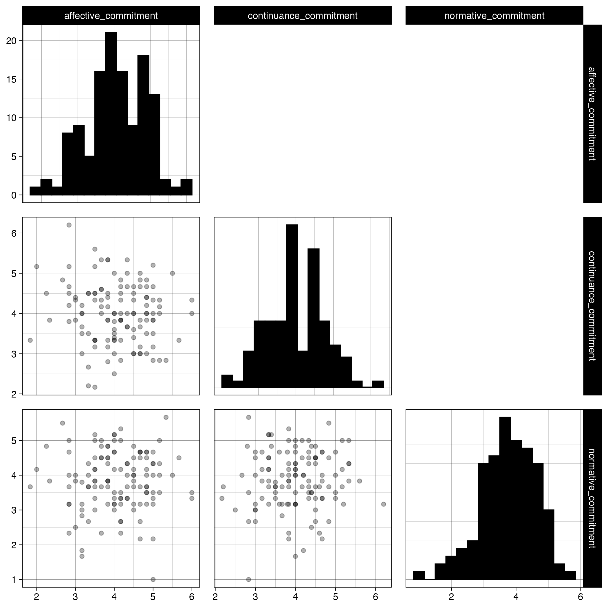
FIGURE 10.2: The pairs plot produced by the pairs_plot_png target.
Stop re-running everything. This is the demonstration that matters. Suppose you change only the analysis — say you tweak the pairs plot. Edit save_pairs_plot() and run tar_make() again:
✔ skipped target raw_file
✔ skipped target imported
✔ skipped target cleaned
✔ skipped target missing_item_csv
✔ skipped target missing_participant_csv
✔ skipped target missing_map_png
✔ skipped target scales
✔ skipped target analytic_final
✔ skipped target cor_table_doc
▶ dispatched target pairs_plot_png
● completed target pairs_plot_png [0.6 seconds]
Everything is skipped except the one target you touched and anything downstream of it. The import, the cleaning, the scale scoring — targets proved they were unaffected and did not redo them. On this project that saves seconds; on a real one it saves hours.
Never wonder what is stale. tar_visnetwork() colours every node by status — up to date or out of date — so the graph itself tells you what is current. And tar_outdated() lists exactly what a rerun would rebuild. You never again have to wonder whether the figure in your manuscript matches your data; the tool tracks it.
10.6.1 Back to reproducibility
Look at what this buys you for the open-science goals from Chapter 7. A reviewer or co-author asks “how was this number produced?” — and the honest, complete answer is now a single sentence: the entire pipeline is tar_make(). The DAG is self-documenting (it shows exactly which target produced each output), the staleness tracking guarantees nothing is out of date, and the whole analysis reruns from raw data with one command. This is precisely the auditable, automatic reproducibility that the TOP guidelines, the FAIR principles, and the Tri-Agency data-management policy are asking for — and it is now a property of your project rather than a promise you have to keep by hand.
10.7 Going further (optional)
targets is the heart of a reproducible project, but three more tools round it out. None is required for this course; treat them as pointers for when your projects grow.
- Version control with
git.gitrecords the history of your project — every change, when you made it, and the ability to go back. Paired with a service like GitHub, it is also how you share a project and how reproducibility checkers get your code. If you learn one thing on this list, learngit. - Robust paths with
here::here(). Instead of fragile paths like"data-raw/data-qualtrics.csv", theherepackage builds paths from your project’s root, so your code works no matter where it is run from. A small habit that prevents a common class of “it works on my machine” failures. - Reproducible package versions with
renv.renvrecords the exact version of every package your project uses, so that years from now (or on a colleague’s computer) the project runs with the same packages it was built with. The final piece of true long-term reproducibility.
targets pipeline: stage functions in R/functions.R, a DAG defined in _targets.R, and the data-interim/ handoffs and master script replaced by targets’ own caching. You watched tar_make() build the pipeline and then skip unchanged targets on a rerun, and you saw tar_visnetwork() draw the same map you sketched by hand. Compare against the my-workflow-project-targets.zip answer key. Nothing is submitted.