Chapter 11 Starting from Scratch
In Chapters 9 and 10 you climbed a ladder. You started with one long script, decomposed it into a structured project, and then orchestrated that project as a targets pipeline. Each step adapted something you already had.
Adapting was the right way to learn, because it showed you the destination — you cannot aim at a clean structure you have never seen. But there is a trap in stopping there, and this chapter is about avoiding it. This is the last hands-on activity of the sequence; as before, you follow along and nothing is submitted.
11.1 Required
This chapter builds a brand-new project on a fresh scenario, plus gives you a reusable template to keep.
| Files |
|---|
| data_job_stress.csv — the fresh toy data set for this chapter |
| project-template.zip — the reusable starter project (copy it for every new study) |
The packages are the ones you already have: tidyverse, janitor, and targets.
11.2 The mindset flip
Here is the trap. Everything you have practised so far is a start-messy-then-clean-up workflow: you began with a working mess and tidied it. That is a genuinely useful skill — you will inherit messy projects your whole career. But real research does not start from a working mess. It starts from an empty folder. If the only mode you have ever practised is “clean up later,” then every new project of your own will begin as a mess that you promise yourself you will fix… eventually. Usually you don’t. The figures pile up, the scripts sprawl, and you are back where Chapter 8 started.
So this chapter teaches the other mode: starting clean. Same destination as before — a targets pipeline with sacred raw data and stage functions — but reached from the beginning rather than retrofitted at the end.
This is the long-promised payoff of begin with the end in mind from Chapter 7. Back then the principle applied to your data and naming — set things up at collection time so analysis is easy later. Now we extend the very same principle to your project structure and code — set the project up, from the first empty folder, already aiming at the clean pipeline. The two modes are worth naming explicitly:
Same destination; different starting point. Once you can start clean, you never have to climb the ladder reactively again.11.3 Design the DAG first
When you adapted a project, you had code first and inferred the DAG from it. Starting clean inverts this: you design the DAG before you write any code. This is the single most transferable greenfield skill in the book, and it is begin-with-the-end-in-mind in its purest form — you decide the shape of the finished pipeline before you build a single piece of it.
The tool is a pencil. Before opening R, sketch the stages and what feeds what. For our new study (described in a moment) the sketch is Figure 11.1: raw data comes in, gets imported, gets cleaned and recoded, gets turned into scale scores, and feeds an analysis that produces a table and a figure.
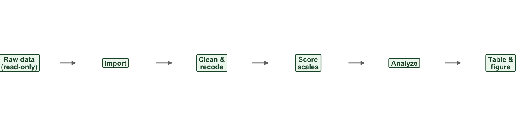
FIGURE 11.1: The DAG for the new study, sketched before any code is written. Design first, build second.
A sketch like this takes two minutes and saves hours. It tells you how many functions you need to write (one per processing box), what each one’s input and output is (read the arrows), and the order everything runs in — all before you have committed to a single line of code. When you do write _targets.R, you are simply transcribing a picture you already have.
11.4 The reusable template and a new-project recipe
The durable artifact you take from this chapter is a project template — a copyable skeleton you reuse for every new study so you never set up the folders by hand again. Download project-template.zip and look inside:
project-template/
├── data-raw/        <- put your raw data here; treat as read-only
├── R/
│   └── functions.R  <- write your stage functions here (starts with naming reminders)
├── output/          <- tables and figures land here
├── _targets.R       <- wire your pipeline here (starts as a skeleton)
└── README.md        <- describe the project for future-you
It is the targets layout from Chapter 10, empty and ready. R/functions.R opens with your naming-convention reminders as comments; _targets.R is a skeleton with the tar_option_set() and tar_source() lines already in place and a commented example target.
With the template in hand, starting a new project is a fixed recipe:
- Copy the template into a new folder named for your study, and open it as an RStudio project.
- Drop your raw data into
data-raw/, and from that moment treat the folder as read-only. - Sketch the DAG on paper (Figure 11.1 is what this looks like).
- Write each processing box as a function in
R/functions.R— inputs in as arguments, one object returned. - Wire
_targets.R— onetar_target()per node, referring to upstream targets by name; the raw data file is aformat = "file"target. - Run
tar_make(), thentar_visnetwork()to confirm the graph matches your sketch. Iterate.
Starting clean is now a repeatable action, not an aspiration. The rest of the chapter walks the recipe twice on fresh ground.
11.5 Worked example: a job-stress study
Imagine a new study, deliberately unlike the commitment survey you have been working with. A research assistant has entered survey data into a spreadsheet for a small workplace study. Each employee reported their department and years employed, answered a four-item job-stress scale (5-point Likert, with one reverse-worded item — “I feel relaxed and calm during my workday”), and answered a three-item turnover-intention scale. The research question: does job stress predict intention to quit?
The raw file is data_job_stress.csv. Note that it is not a Qualtrics export — there are no three header rows, no junk columns. It is a clean spreadsheet typed by a person. This matters: it is exactly why we design from scratch rather than reuse the Qualtrics functions wholesale. The skills transfer; the specific code adapts.
11.5.1 Step 1–3: copy the template, add data, sketch
Copy the template to a folder called job-stress-study, drop data_job_stress.csv into data-raw/, and sketch the DAG. The sketch is Figure 11.1 — it is short, because this is a smaller study. Six boxes, five arrows, one fan-out at the end (the analysis produces both a table and a figure).
11.5.2 Step 4: write the stage functions
Now write one function per processing box, into R/functions.R. Each follows the rule from Chapter 10: inputs in as arguments, one object returned.
The import step is simpler than the Qualtrics one — a spreadsheet needs no header-skipping and no junk-column removal — and in fact the template already ships exactly this generic importer as import_data(), so here you reuse it as-is:
import_data <- function(survey_file) {
  readr::read_csv(survey_file, show_col_types = FALSE, na = c("", "NA")) |>
    clean_names() |>
    remove_empty("rows") |>
    remove_empty("cols") |>
    mutate(participant_id = row_number()) |>
    relocate(participant_id)
}
The clean-and-recode function makes department a factor and handles the Likert items. The one wrinkle that needs real work is the reverse-keyed item — and notice the arithmetic differs from the commitment study. These are 5-point items, so a reverse-keyed response is subtracted from 5 + 1 = 6 (in Chapter 10 the 7-point items used 7 + 1 = 8). This is the kind of detail your sketch and naming convention keep straight for you: the _likert5rev suffix tells you both that the item is reversed and that the scale has five points.
clean_recode_jobstress <- function(data) {
  data <- data |>
    mutate(department = as_factor(department))

  likert5_recode <- c(
    "Strongly Disagree" = 1, "Disagree" = 2, "Neutral" = 3,
    "Agree" = 4, "Strongly Agree" = 5
  )

  data <- data |>
    mutate(across(.cols = contains("likert5"), .fns = ~ likert5_recode[.x]))

  # Reverse-key the 5-point item: subtract from 5 + 1 = 6, then drop the suffix
  data |>
    mutate(across(.cols = ends_with("_likert5rev"), .fns = ~ (5 + 1) - .x)) |>
    rename_with(.fn = ~ str_replace(.x, "_likert5rev", "_likert5"),
                .cols = ends_with("_likert5rev"))
}
The scale-scoring function averages each set of items into a score and drops the items. Because the items were named with unique prefixes (jstress..., turn_int...) and the scales with different prefixes (job_stress, turnover_intention), starts_with() selects exactly what we want — the same careful naming discipline from Chapter 7:
create_scales_jobstress <- function(data) {
  data |>
    rowwise() |>
    mutate(
      job_stress         = mean(c_across(starts_with("jstress")),  na.rm = TRUE),
      turnover_intention = mean(c_across(starts_with("turn_int")), na.rm = TRUE)
    ) |>
    ungroup() |>
    select(-starts_with("jstress"), -starts_with("turn_int"))
}
Finally, two analysis functions — one for a correlation table, one for the scatterplot — each taking a path and returning it, so a format = "file" target can track the output:
save_jobstress_table <- function(scores, path) {
  apaTables::apa.cor.table(
    scores |> select(job_stress, turnover_intention),
    filename = path, table.number = 1
  )
  path
}

save_jobstress_plot <- function(scores, path) {
  p <- ggplot(scores, aes(x = job_stress, y = turnover_intention)) +
    geom_point(alpha = 0.5) +
    geom_smooth(method = "lm", formula = y ~ x) +
    labs(x = "Job stress", y = "Turnover intention") +
    theme_classic(14)
  ggsave(path, plot = p, width = 6, height = 4.2, dpi = 300)
  path
}
11.5.3 Step 5: wire _targets.R
With the functions written, _targets.R is a direct transcription of your sketch — one tar_target() per box, each referring to the previous target by name:
# _targets.R
library(targets)

if (!dir.exists("output")) dir.create("output")

tar_option_set(packages = c("tidyverse", "janitor", "apaTables"))
tar_source("R/functions.R")

list(
  tar_target(raw_file, "data-raw/data_job_stress.csv", format = "file"),
  tar_target(imported, import_data(raw_file)),
  tar_target(cleaned,  clean_recode_jobstress(imported)),
  tar_target(scores,   create_scales_jobstress(cleaned)),
  tar_target(cor_table,
             save_jobstress_table(scores, "output/table-stress-turnover.doc"),
             format = "file"),
  tar_target(scatter_png,
             save_jobstress_plot(scores, "output/figure-stress-turnover.png"),
             format = "file")
)
11.5.4 Step 6: build and check
Run the pipeline and draw it:
tar_visnetwork() will draw a graph that matches the sketch in Figure 11.1 — confirmation that what you built is what you designed. The pipeline produces a correlation table and Figure 11.2: job stress is strongly, positively related to turnover intention. (One participant who left the survey blank produces missing scale scores and drops out of the figure — exactly the kind of thing a missing-data stage, like the one in Chapter 10, would flag; adding one here is a natural extension.)
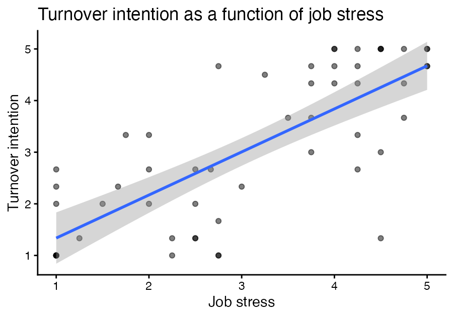
FIGURE 11.2: The relationship between job stress and turnover intention, produced by the from-scratch pipeline.
That is a complete project, built clean from an empty folder, with no mess to clean up afterwards. You designed the DAG, copied the template, wrote one function per node, wired the pipeline, and ran it.
11.6 A second walkthrough
Let us run the recipe once more, on different ground, so the pattern sticks. New scenario: a training study. Employees completed a brief perceived-organizational-support (POS) scale — three 5-point items, one reverse-worded — and you have a single outcome already recorded numerically, weekly training hours. The question: does perceived support predict how much optional training people take on? Imagine the raw spreadsheet is data_training.csv in the same clean, RA-entered format, with items named pos1_likert5, pos2_likert5, pos3_likert5rev, and a numeric training_hours column.
Walk the recipe:
1–3. Copy, add data, sketch. Copy the template to training-study, drop the raw file into data-raw/, and sketch. The DAG is even shorter than the last one — there is only one scale to score, and the outcome is already numeric:
raw_file → imported → cleaned → scores → analysis (table + figure)4. Write the functions. The import function is the same shape as before (it is the generic spreadsheet importer — notice how reusable that step is). The clean-recode function needs only the 5-point recode and the single reverse-keyed item:
clean_recode_training <- function(data) {
  likert5_recode <- c(
    "Strongly Disagree" = 1, "Disagree" = 2, "Neutral" = 3,
    "Agree" = 4, "Strongly Agree" = 5
  )
  data |>
    mutate(across(.cols = contains("likert5"), .fns = ~ likert5_recode[.x])) |>
    mutate(across(.cols = ends_with("_likert5rev"), .fns = ~ (5 + 1) - .x)) |>
    rename_with(.fn = ~ str_replace(.x, "_likert5rev", "_likert5"),
                .cols = ends_with("_likert5rev"))
}
The scoring function builds the one POS scale. There is no scale to build for the outcome — training_hours is already a number, so we simply leave it alone:
create_scales_training <- function(data) {
  data |>
    rowwise() |>
    mutate(pos = mean(c_across(starts_with("pos")), na.rm = TRUE)) |>
    ungroup() |>
    select(-starts_with("pos_"))   # drop the items, keep the pos scale
}select(). The items are named pos1_likert5, pos2_likert5, … and the scale is named pos. If we had written select(-starts_with("pos")) we would have deleted the scale we just built! We use starts_with("pos_") (with the underscore) so it matches the items but not the bare pos scale. This is precisely the naming-and-selection care Chapter 7 warned about, and it bites in every new project — which is why the recipe puts “design and name carefully” before “write code.”
The analysis function follows the same save_<study>_table() pattern as the first walkthrough — only the columns it selects change, because here we correlate the pos scale with the numeric training_hours outcome:
save_training_table <- function(scores, path) {
  apaTables::apa.cor.table(
    scores |> select(pos, training_hours),
    filename = path, table.number = 1
  )
  path
}
5. Wire _targets.R. Again, a transcription of the sketch:
list(
  tar_target(raw_file, "data-raw/data_training.csv", format = "file"),
  tar_target(imported, import_data(raw_file)),               # the generic importer, reused
  tar_target(cleaned,  clean_recode_training(imported)),
  tar_target(scores,   create_scales_training(cleaned)),
  tar_target(cor_table,
             save_training_table(scores, "output/table-pos-training.doc"),
             format = "file")
)
6. Build and check. tar_make(), then tar_visnetwork() to confirm the graph matches the sketch.
Notice what happened across the two walkthroughs: the recipe never changed, and several functions (the spreadsheet importer especially) carried straight over. Starting clean is not more work than starting messy — it is the same work, done in an order that leaves you with a clean project instead of a cleanup chore. That reuse is the reuse your work payoff from Chapter 9, arriving exactly when you start clean from the template.
11.7 Where you have arrived
Step back and take in the whole arc. You began, in Chapter 8, with a single long script. You learned to decompose it into a structured project (Chapter 9), to orchestrate that project as a self-maintaining targets pipeline (Chapter 10), and now to start a new project clean from an empty folder, aiming at that destination from the first day.
The road map that opened as an abstract concept in Chapter 7 is now something you can build with your hands, have the computer draw and maintain for you, and design from scratch before writing a line of code. That is what begin with the end in mind was always pointing toward — and it is the foundation your future research, at whatever scale, will stand on.
targets project from an empty folder for a fresh job-stress study — designing the DAG first, writing one function per node, and confirming the built graph matched your sketch — and then walked the same recipe a second time on a training study. Keep the project-template.zip: it is the starting point for every project you build from here on. Nothing is submitted.